Since the original "Attention is All You Need" paper started the Transformer craze in the NLP community, it seems like we've been in relentless pursuit of larger models and marginally lower perplexities. In the summer of 2019 NVIDIA released their MegatronLM paper – weighing in at 8.3B parameters. In February of 2020 Microsoft upped the ante again, releasing a blog post on Turing-NLG and boasting 17B parameters.
Now there certainly is value in understanding how our current methods scale as we increase the number of parameters and the amount of training data these models have access to, and I'm happy that organizations with the resources to conduct these large-scale experiments have done so. However, comparatively little time and energy has been spent understanding how we can adapt the Transformer architecture to make it more efficient.
"Reformer: The Efficient Transformer" by Nikita Kitaev, Łukasz Kaiser, Anselm Levskaya is in sharp contrast to the "bigger is better" trend of the past two years, and was accepted for a talk at ICLR 2020. The Reformer paper reads like a breath of fresh air – focusing primarily on how the self-attention operation scales with sequence length, and proposing an alternative attention mechanism to incorporate information from much longer contexts into language models.
With the Reformer's changes to the Transformer, they're able to attend over sequences up to 64,000 tokens in length on a single accelerator – which is in sharp contrast to the 1024 token context size of MegatronLM and TuringNLP, both of which used pipeline model parallelism to cope with their massive parameter counts.
A Review of Self-Attention
Let's briefly review the formulation of self-attention before we dive into the details of the Reformer architecture to get some context for the obstacles standing in the way of incorporating long-term context.
For purposes of simplicity, we'll speak about dot product attention with a single head, although multiple attention heads are used in practice.
If you want a more in-depth review of the self-attention mechanism, I highly recommend Alexander Rush's Annotated Transformer for a dive into the code, or Jay Alammar's Illustrated Transformer if you prefer a visual approach.

We can break down self-attention into three main parts:
Query - Key - Value Projection

In this stage the current hidden state for each token is broken up into three components via a linear projection.
queries = np.matmul(query_weights, hidden) + query_bias
keys = np.matmul(key_weights, hidden) + key_bias
values = np.matmul(value_weights, hidden) + value_bias
Query / Key Matrix Multiply

After the projection, queries and keys are multiplied to compute a measure of agreement. This is implemented as a matrix multiply.
qk_agreement = np.matmul(queries, np.swapaxes(keys, -1, -2))If your keys and queries are tensors of shape (batch, sequence_length, hidden_size), the output of the matrix multiply is a tensor of shape (batch, sequence_length, sequence_length).
This seemingly innocuous matrix multiply is the source of the self-attention operation's computational complexity issues. For a linear increase in sequence length, the number of multiplications required to compute our output increases quadratically, because we compute a scalar measure of agreement for every possible pair of tokens in our input. This O(L²) complexity means that sequence lengths of longer than 1024 tokens quickly become impractical using a vanilla transformer architecture. In fact, BERT and it's successor RoBERTa opted for a context length of only 512.

Softmax + Weighted Sum of Values
By convention, the entries in the key / value agreement matrix are divided by a scalar factor of sqrt(hidden_size) to help with parameter flow and to help decouple the sharpness of our attention distribution from our hidden size hyperparameter. For each query we compute a softmax over all keys to ensure that each row of our matrix sums to one – ensuring the magnitude of our new hidden state does not depend on our sequence length. Finally, we multiply our attention matrix by our matrix of values to produce a new hidden representation for every token.
attention_weights = softmax(qk_agreement / qk_agreement.shape[-1])
attention_outputs = np.matmul(attention_weights, values)
Computational Complexity – Solutions
Like mentioned previously, although the dot product attention formulation is quite expressive and allows any token within our context to aggregate information from any other token at each layer, this flexibility comes at a cost of an unfortunate O(L²) computational complexity term.
Several papers have proposed transformer variants that help address this computational complexity. "Generating Long Sequences With Sparse Transformers" suggests factorizing the attention operation using pairs of attention operations with carefully selected attention patterns. "Transformer-XL: Attentive Language Models Beyond a Fixed-Length Context" introduces a recurrent mechanism to allow for incorporating information from distances larger than the the self-attention operation's context size.
The Reformer
The authors of "Reformer: The Efficient Transformer" take an entirely different approach to tackling the sequence length issue. First, they observe that learning different projections for keys and queries are not strictly necessary. They toss out the query projection and reframe the attention weights as a function of key agreement.

Somewhat surprisingly, though they've removed some parameters from the attention block, the performance of their model does not degrade on enwiki8.
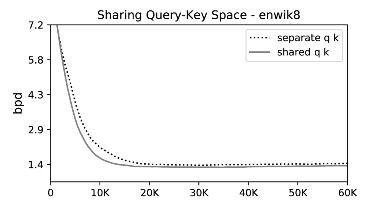
Now that the attention block no longer contains a separate projection for queries, we have only our key and value pairs. Computing the key agreement matrix (by comparing each key to every other key) is still equally expensive, however.
This is unfortunate because we likely aren't taking advantage of all of this computation. The softmax outputs are typically dominated by a few key elements – the rest tend to wash out in the noise. We don't necessarily get richer representations of our tokens by incorporating information from the tokens that produced small attention weights for a given token.
When writing traditional software, we run into a flavor of this problem all the time. If we want to find a value that corresponds to a given key, we typically don't iterate over a list of all keys and check each to see if we have a match. Instead, we use hash map data structures to do O(1) lookups rather than O(n) comparisons.
Conveniently, an analogue to hash maps for vector spaces does exist, and it's called "locality sensitive hashing" (LSH). It's to this method that the authors of the Reformer paper look to produce a transformer alternative that avoids the quadratic complexity of dot product attention.
Locality Sensitive Hashing (LSH)
Locality sensitive hashing is a family of methods that map high dimensional vectors to a set of discrete values (buckets / clusters). It's most commonly used for as a method for approximate nearest neighbor search, for applications like near duplicate detection or visual search.
Locality sensitive hashing methods try to assign vectors that are close in their high dimensional space to the same hash with high probability. There are a wide range of valid hash functions, but perhaps the simplest involves random projections.
lsh_proj = np.random.randn(hidden_size, hash_size)
hash_value = np.sign(np.dot(x, lsh_proj.T))
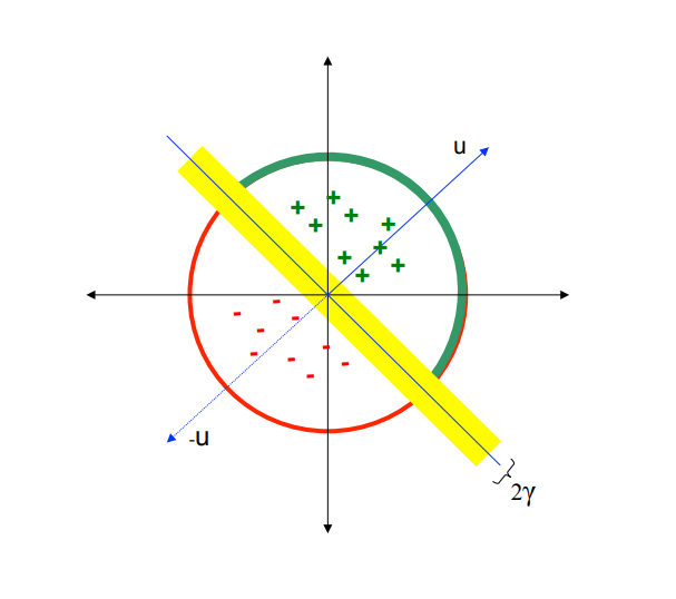
In other words, we select a random set of vectors, observe whether the projection of the input vector onto each is positive or negative, and use that vector of bits to indicate the intended bucket for a given vector. The diagram below illustrates that process for a single vector in the LSH projection matrix, "u". The green plus marks indicate points that had a positive dot product with our vector u, while the red minus signs indicate points that produced a negative value.
LSH Attention
The Reformer paper opted to use an angular variant of locality sensitive hashing. They first constrain each input vector's L2 norm (i.e. – project the vector onto a unit sphere), then apply a series of rotations, and finally find the slice that each rotated vector belongs to.
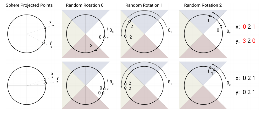
Finding the slice that a given vector belong to after rotation can also be viewed as finding the vector with which the input is most aligned – the procedure outlined in code below paraphrased from the Reformer's source code:
# simplified to only compute a singular hash
random_rotations = np.random.randn(hidden_dim, n_buckets // 2)
rotated_vectors = np.dot(x, random_rotations)
rotated_vectors = np.hstack([rotated_vectors, -rotated_vectors])
buckets = np.argmax(rotated_vectors, axis=-1)
After computing a bucket for each token, the tokens are sorted according to their bucket and standard dot-product attention is applied to chunks of the bucketed tokens.
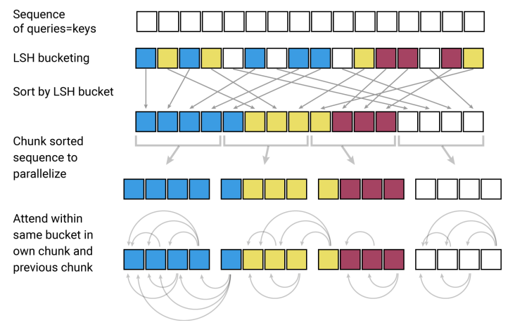
With a sufficient number of buckets, this dramatically shrinks the number of tokens that any given token is required to attend to – on experiments the Reformer paper ran the model was configured to use a chunk size of 128. So the LSH operation serves to limit the context size of the expensive key agreement matrix multiply to a more manageable value.
Instead of having time complexity proportional to O(L²), we now have time complexity proportional to O(L*log(L)) – which allows us to tractably extend the attention operation to much longer sequences without being crippled by runtime.
Because this bucketing process is stochastic, the Reformer authors optionally run this process several times to reduce the possibility of two vectors that are close in input space from being placed in disparate buckets by random chance. When all is said and done, you have a drop-in replacement for standard multi-head attention that's competitive with computing the full attention matrix.
Memory Complexity
Unfortunately, achieving better time complexity is only half the problem. If we swapped our new LSH attention block in for the standard multi-head attention and tried to feed in novel-length inputs, we'd quickly realize the next bottleneck in the system – memory complexity.
Even though we've taken great care to minimize the computational complexity of the attention operation, we still have to store all our keys and values in memory! Even worse, during training we need to cache our activations in order to compute our parameter updates.
The Reformer paper uses a sequence length of 64k tokens for experiments on the enwiki8 language modeling dataset -- with a hidden size of 1024 and 12 layers this means storing our keys and values alone requires 2 * 64,000 * 1024 * 12 = ~1.5B floating point numbers, or over 6GB of device memory per example for single-precision floats. With this kind of memory usage, we'll be unable to use large batch sizes during training and our runtimes will suffer as a result.
One option would be to implement gradient checkpointing to help limit our memory usage. Gradient checkpoints allow us to reduce memory use by storing only key activations from the forward pass and recomputing the rest during the backward pass. So instead of storing our keys and values, we could choose to only store the hidden state prior to the keys and value projection, and re-project our hidden states a second time to compute our gradients.
This unfortunately doubles the cost of our backward pass, so the gains we'd get from being able to support larger batch sizes would be partially mitigated by the re-computation. More importantly, even if we choose to only store a fraction of the inputs, the fact that storing a single layer's activations requires 250MB of space means we'd be hard pressed to support batch sizes of more than around dozen examples on a 12GB GPU.
RevNets
Fortunately, we have other options to reduce our memory use. Enter the Reversible Residual Network – RevNet for short.
In a clever computational trick, RevNets keep memory use constant with the depth of the network by structuring each layer in a particular way. Each layer is split into two components, X₁ and X₂, and the forward pass in computed as follows:
def forward_pass(x1, x2, Wf, Wg):
    """
    Need an extra node in the computational graph
    because the gradient of the loss with respect to z1       # differs from the gradient of loss with respect to y1
	x1: one half of layer input
    x2: other half of layer input
    Wf: weights that parameterize function f
    Wg: weights that parameterize function g
    """
    z1 = x1 + f(Wf, x2)
    y2 = x2 + g(Wg, z1)
    y1 = z1
Visually, this looks like:

Because of the layer's specific structure, we can write a custom parameter update routine that means we don't have to cache any activations to compute our backwards pass! Similar to using gradient checkpointing, we still have to do some redundant computation. However, because every layer's inputs can be easily constructed from it's outputs, our memory use no longer scales with the number of layers in the network.
# paraphrased from the RevNet paper

def backward_pass(y1, y2, d_y1, d_y2, Wf, Wg):
    """
    Pseudocode for RevNet of backward pass

    y1: one half of layer output
    y2: second half of layer output
    d_y1: derivative of y1
    d_y2: derivative of y2
    Wf: weights that parameterize function f
    Wg: weights that parameterize function g
    """
    z1 = y1

    # Extra computation -- the price we pay for memory
    # complexity that doesn't scale with n_layers
    # Importantly this means we don't have to store x1 or x2!
    x2 = y2 - g(Wg, z1)
    x1 = y1 - f(Wf, x2)

    # Standard backprop:
    # vjp --> Vector Jacobian Product
    d_Wf, partial_x2 = jax.vjp(f, Wf, x2)(d_z1)
    d_Wg, partial_z1 = jax.vjp(g, Wg, z1)(d_y2)
    d_z1 = d_y1 + partial_z1
    d_x2 = d_y2 + partial_x2

    d_x1 = d_z1

    return x1, x2, d_x1, d_x2, d_Wf, d_Wg
In practice, the Reformer defines f(x) to be the LSH Attention block and g(x) to be the standard feed forward block from the transformer architecture.
With the RevNet architecture in place, we only need to store a single layer's activations in memory and we can use substantially larger batch sizes during training! Now that we're no longer crippled by the memory footprint of our activations during training, we're able to take advantage of the time complexity improvements of the LSH Attention block!
Importantly, language model loss does not degrade because of unique reversible layer structure that is imposed.
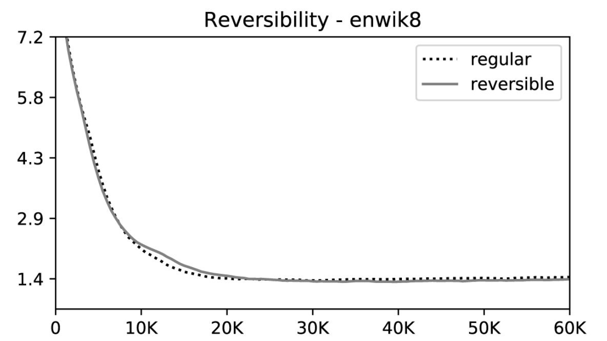
These changes are by no means simple to implement -- it's clear Nikita Kitaev, Łukasz Kaiser, and Anselm Levskaya put a herculean amount of effort into this balancing act of time and memory, and I encourage you to marvel at the software engineering effort behind the reformer paper.
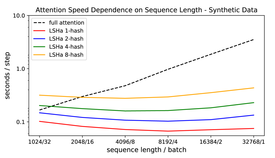
In combination, these changes enable some rather impressive scaling with respect to sequence length (below). Although results are preliminary, experiments on enwiki8 also suggest that the Reformer may well be capable of competing with it's heavier weight predecessor on language modeling tasks -- a 12-layer Reformer with hidden size 1024 yields 1.05 bits/dim on the task.
Conclusion
Locality sensitive hashing-based attention and reversible layers form the basis of the Reformer's blueprint for a more efficient transformer, and it's exciting to see work on transformer based architectures that chooses to optimize for handling long sequence lengths rather than simply scaling up prior work in the hunt for marginally lower perplexities.
If you're interested in tracking future work by Nikita Kitaev, Łukasz Kaiser, and Anselm Levskaya, drop by and say hello in the Trax gitter community! I'm eagerly awaiting their follow-up experiments on machine translation tasks and am interested to see what wild applications the community finds for this novel architecture.


