
In keeping with the theme of "conditional-computation" I've been exploring with recent blogs posts on the Reformer, Routing Transformer, and Sinkhorn Transformer, I took some time this weekend to read the 2019 paper "Large Memory Layers with Product Keys" by Guillaume Lample, Alexandre Sablayrolles, Marc'Aurelio Ranzato, Ludovic Denoyer, and Hervé Jégou of Facebook AI Research. "Large Memory Layers with Product Keys" describes an efficient, nearest-neighbors method for allowing a language-model to query a large memory matrix for specific information. Compared to vanilla transformers that achieve similar perplexities through additional layers, shallower models equipped the large memory layers are twice as fast.
Motivation
I'm wary of drawing too detailed of a comparison to the brain, but I think an analogy is warranted to motivate the use of disparate kinds of computation in natural language processing models. As humans, the process of recalling a specific fact or event feels nearly instantaneous. Any owner of a brain can attest that recalling specific memories doesn't require an exhaustive linear search through past memories.
Certain kinds of knowledge (syntax, grammar, etc.) are accessed every time we form an sentence. Other varieties of knowledge (for instance, that giraffes have the same number of vertebrae in their neck as we do) are much less frequently useful. It's only natural that the mechanisms we use to represent these two distinct kinds of information in neural networks differ.
Memory Matrix
Let's say we wanted to design a neural network analogue to long-term memory. We might think about modeling facts / memories as a matrix, where each vector in the matrix represents a specific piece of information. However, this information is only infrequently relevant – we only want to access each vector when it is useful (sparse memory access). Additionally, storing a large amount of specific information necessitates a large matrix. This is in contrast to typical settings where we want to learn parameters that are general purpose and used frequently.
Query Strategies
Vanilla dot product attention, where we dot the query vector with every key in order to produce a measure of key-query agreement, is an exceptionally poor fit for this scenario. Since dot product attention has linear complexity with respect to the number of stored items, increasing the size of our memory matrix is quite costly and quickly becomes intractable. So how might we go about designing computational building blocks that don't scale linearly with memory size?
Some of my previous blog posts have focused on a similar problem of allowing attention between tokens that are distant from each other in an input document. The Reformer suggests a solution based on locality sensitive hashing, where the latent space is partitioned up and information flow is allowed between elements contained within the same partition. The Routing Transformer takes inspiration from the K-means clustering algorithm, and allows attention within a given cluster. The Sinkhorn Transformer looks to the field of optimal transport and differentiable sorting for inspiration, and attends locally over a sorted view of a sequence. They all suggest mechanisms for performing selective computation – rather than allowing dense interaction between every element in the sequence they describe methods for sharing information only between relevant subsets of the sequence.
Similar to these methods designed for long-term attention, "Large Memory Layers with Product Keys" lays out a mechanism the authors term "Product-Key Memory" for selectively accessing values in a large matrix, this time based on a decomposed nearest-neighbors computation.
Parameter Count vs. Runtime Complexity
Runtime complexity and parameter count are often conflated, and drawing comparisons between models of similar parameter counts is generally accepted as a practice for ensuring a "fair" comparison of two model architectures. Yet parameter count is rarely the true limiting factor – modern GPUs have more than enough memory to store all but the largest models, and storing model activations (rather than model weights) typically requires more GPU memory at training time. So efficient mechanisms that enable the use of more parameters through conditional computation hold real promise as practical options for lowering perplexity without significantly increasing prediction time.
Architecture
The architectural contribution of "Large Memory Layers with Product Keys" has three primary components – a query network, a key selection component, and a value lookup table.
The query network is analogous to the query projection in self-attention – it could be as simple as the linear projection of the hidden state using in self-attention or could be parameterized by a small MLP.
Next up is the problem of key-selection. At the heart of this problem is an efficient nearest-neighbors query to find keys that correspond closely to a given query. Methods to enable faster generic nearest-neighbor computation typically involve some sort of hierarchical partitioning scheme (KD-trees, for instance) or lossy approximation of the true nearest neighbors. However, a key insight is that in this scenario we have control over the process that produces our keys. We can exploit this to structure our keys in a way that enables faster exact queries using "product-keys".
Product-Key Memory
Let's look at the expansion of the dot-product (measure of agreement) between two \(d\) dimensional vectors, \(q\) and \(k\).
$$ qk = q_1 k_1 + q_2 k_1 + ... + q_d k_d $$
We would like to compute agreement for \(n\) keys – but importantly, we get to pick the structure of our keys. What if we considered each value \(k_i\) to be the concatenation of two vector components, \(c\) and \(c'\)? If we have \(\sqrt{n}\) vectors for \(c\) and \(c'\), we can produce \(n\) unique keys.
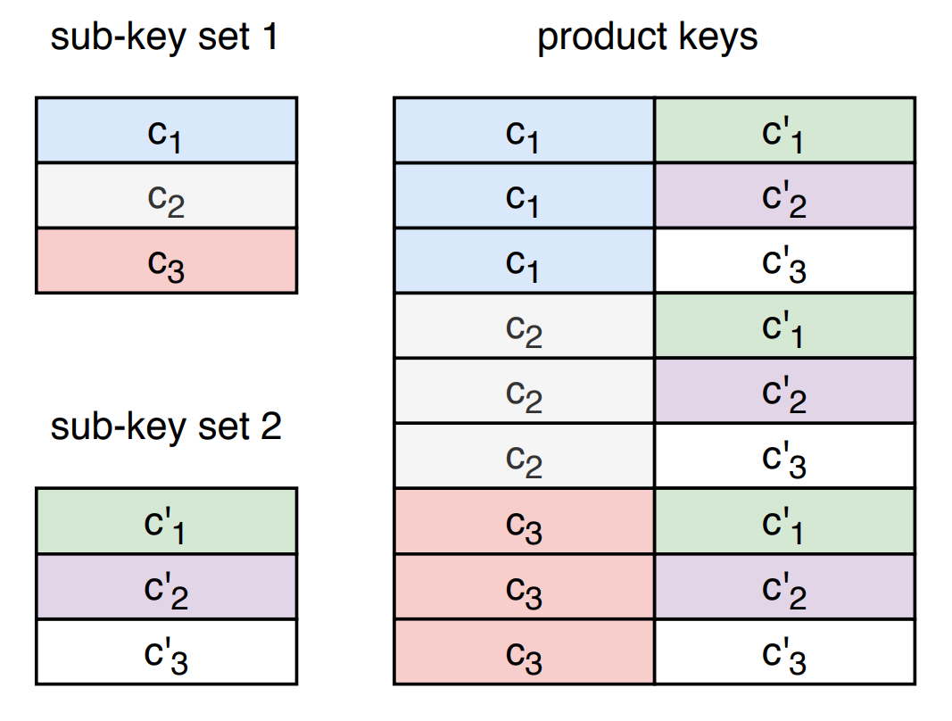
If we denote the two corresponding halves of our query vector as \(b\) and \(b'\), then we can re-write our distance computation for a given query / key pair using the sum of the two halves.
$$ qk = (b_{1} c_{1} + ... + b_{d/2} c_{d/2}) + (b'_{1} c'_{1} + ... + b'_{d/2} c'_{d/2}) $$
Because of how the product keys are constructed, instead of having to compute \(n\) distances, we need only compute \(\sqrt{n}\) dot products between \(b\) and \(c\), and another \(\sqrt{n}\) dot products between \(b'\) and \(c'\). This provides us with all the necessary information to compute the dot products of full set of keys via a simple addition of each keys 2 components' dot-products.
Complexity
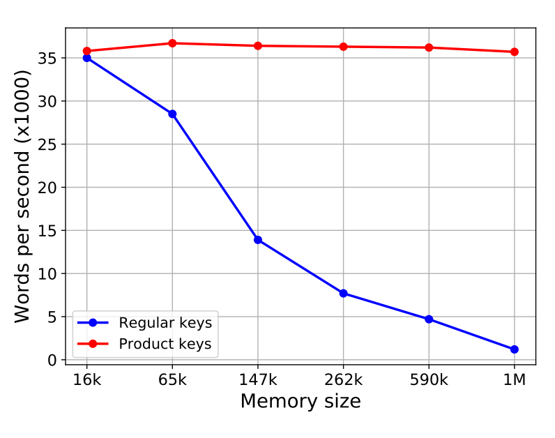
Although the illustration above uses \(n=9\), a value of \(512^2\) was used in the paper's primary experiments. A naive dot product between a query vector and \(512^2\) keys of dimension \(d\) would typically require \(512^2*d\) multiplications. In comparison, the product-key method requires only \(512 * d\) multiplications. Generically, the runtime complexity of the product-key method is \(O(d\sqrt{n})\).
Candidate Pool Generation and Filtering
If we then take the top \(k\) elements of the first comparison, and the top \(k\) elements of the second comparison, we can produce a candidate pool of \(k^2\) keys by selecting all keys that contain elements from both sets (the cartesian product). Our candidate pool is guaranteed to include the exact top \(k\) matching keys as our key score is proportional to the sum of the two component-wise scores. Because \(k\) is small by design, iterating over the \(k^2\) keys to find the top \(k\) matches is sufficiently efficient.
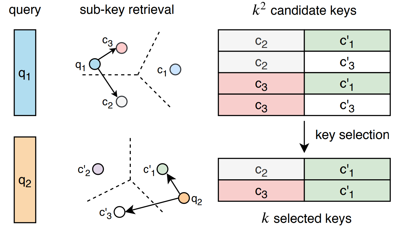
Also important is that the key matrix never needs to be instantiated – operations performed on \(c\) and \(c'\) allow us to determine which keys to access without ever explicitly constructing the key matrix.
A Brief JAX Implementation
For those who prefer python to mathematics, the key portion of the product-key memory layer is below. A full pytorch implementation of the product-key memory is also available as portion of Facebook's XLM repository.
def product_key_layer(query, subkeys, top_k=32):
    """
    query: [batch_size, hidden_dim]
    subkeys: [2, hidden_dim / 2, n_keys]
    """
    batch_size, hidden_dim = query.shape
    _, half, n_keys = subkeys.shape
    q1 = query[:, :half]
    q2 = query[:, half:]

    # Linear projection to get scores per subkey
    scores1 = np.matmul(q1, subkeys[0])
    scores2 = np.matmul(q2, subkeys[1])

    # Take top-K entries of each score array
    batched_top_k = vmap(lax.top_k, in_axes=(0, None))
    top_scores1, top_indices1 = batched_top_k(scores1, top_k)
    top_scores2, top_indices2 = batched_top_k(scores2, top_k)

    # Produce [batch_size, top_k * top_k]
    # matrix of full key scores
    # via broadcast-sum (cartesian product)
    all_scores = (
        np.expand_dims(top_scores1, 2) +
        np.expand_dims(top_scores2, 1)
    ).reshape(batch_size, top_k * top_k)

    # Corresponding indices into our
    # structured key matrix
    all_indices = (
        np.expand_dims(top_indices1, 2) * n_keys +
        np.expand_dims(top_indices2, 1)
    ).reshape(batch_size, top_k * top_k)

    # True top_k scores selected from candidate pool
    # and corresponding indices into top_k^2 array
    scores, local_indices = batched_top_k(all_scores, top_k)

    # Translating candidate indices back
    # to indices into full value array
    indices = np.take(all_indices, local_indices, axis=1)
    return scores, indices
Using the Selected Indices for Sparse Attention
Once the top \(k\) keys have been selected for a given query, all that's left is to attend over the selected subset and take a weighted average of the corresponding values to produce the output hidden state. Below, \(x_i\) denotes a dot-product score between a query / key pair from the top \(k\) keys.
$$ w_i = \frac{e^{x_i}}{\sum_{j=0}^{k} e^{x_j}} $$
$$ X = \sum_{i=0}^{k} w_i V_i $$
Similar to attention, this process could be broadcast across \(H\) heads to query \(H\) sets of \(k\) values, and the author's find that the multi-head variant of this process aids language modeling performance.
Piecing this altogether, the computation performed by the large memory layer looks like the diagram below:
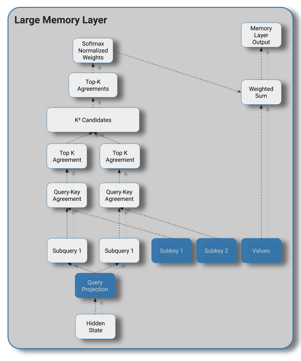
Although we could place this layer anywhere, the author's elect to substitute the feed forward network of select layers with the large memory layer.
Experimental Results
The Product-Key Memory (PKM) Layer performs well in practice when applied at scale. Rather than evaluating the large memory layer method on many of the smaller traditional language modeling benchmarks (enwiki8, text8), the authors opt to benchmark using a 28 billion word (40 million new article) subset of the Common Crawl corpus. The decision to use a larger corpus seems reasonable given that the product-key memory will be sparsely accessed and may require more updates than a typical transformer model to learn good representations for the values in the memory layers.
Lample et. al make a strong case for product-key memory having disproportionate impact per unit runtime cost – a 12 layer model with 2 PKM layers produces test scores about 1.2 PPL lower than a corresponding 24 layer model with no PKM layers at 1.75x the throughput!
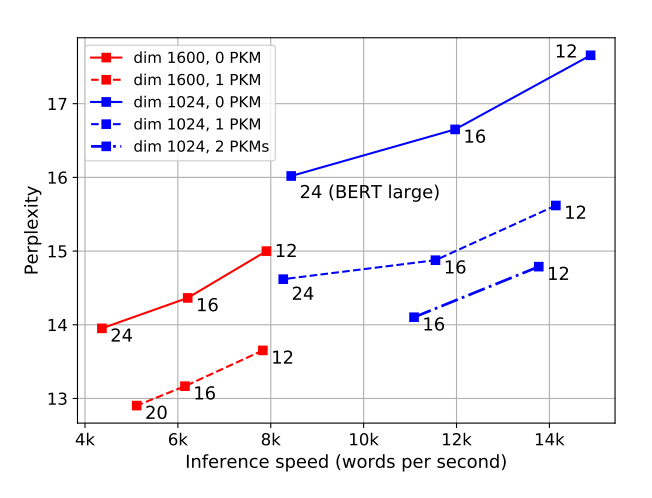
They also demonstrate that the size of the product-key memory layer can be increased at negligible cost – meaning making use of larger memory stores is primarily a matter of ensuring sufficient training data availability to learn meaningful representations for the sparsely accessed values.
Ablations:
Somewhat counter-intuitively, the parameter sharing of the product key structure leads to better perplexities than baselines with a flat key structure. The authors suggest this delta is attributable to better key-utilization – with a flat key structure at 147k keys only 10% of keys are used at least once (compared to 100% utilization with product-keys).
Likewise the application of batch norm at the output of the query network seems critical for good perplexities – networks without batch norm utilize a smaller percentage of total keys when the key count exceeds 100k.
Closing Thoughts
Although the simplicity of the transformer architecture is appealing I strongly believe there's a need to mix in components with a diverse set of inductive biases to continue to make progress in language modeling. Product-key memory seems like a strong contender for sparsely accessed memory, and I'm looking forward to future work by Guillaume Lample, Alexandre Sablayrolles, Marc'Aurelio Ranzato, Ludovic Denoyer, and Hervé Jégou.
Feel free to reach out to madison@indico.io if you find any typos or inaccuracies – my blog posts are living documents and I'm always happy to receive constructive feedback.