This week I'm diving into "Sparse Sinkhorn Attention" by Yi Tay, Dara Bahri, Liu Yang, Donald Metzler, and Da-Cheng Juan. "Sparse Sinkhorn Attention" uses the concept of differentiable sorting to construct an attention algorithm with memory complexity that scales approximately linearly with sequence length.
Although Sparse Sinkhorn Attention was published in 2020, to properly understand the paper's key contribution – and to describe how the author's were able to define a differentiable sorting operation – we're first going to take a trip back in time to understand optimal transport and the Sinkhorn-Knopp algorithm.
Optimal Transport
Optimal transport is a mathematical concept dating back to 17th century France and the mathematician Gaspard Monge, who described the problem of efficiently moving a mound of sand to fill a sinkhole of equal volume. Intuitively, moving each discrete shovel-full of sand takes a defined amount of effort – for instance, a product of the weight of the sand and the distance moved (our local cost). Optimal transport involves the computation of the transport strategy with the lowest total (global) cost.
In machine learning, we often see optimal transport surface in contexts where we would like to compute how to transform one distribution into another. Rather than moving a mountain of sand to fill a sinkhole, we might be concerned with understanding the transport between two probability distributions, for instance.
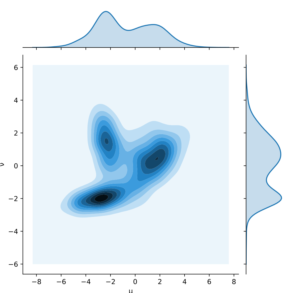
Although the image above depicts two continuous probability distributions, for most practical applications we instead have discrete distributions – for example, the distribution over class probabilities in the context of a classification problem.
Toilet Paper Distribution as Optimal Transport
Let's consider for a moment a physical example – imagine for a moment you are in charge of logistics for a giant manufacturing operation at Charmin. You have industrial machines at 5 factories cranking out that luxurious 2-ply as fast as possible and you need to distribute the Charmin Ultra-Soft to 5 regional distribution centers as efficiently as possible to deal with the current COVID-19 induced toilet paper shortage.
Each factory is capable of different rates of production, and each region has different demand, so you can't simply source Charmin Ultra-Soft from the factory nearest each regional distribution center. In addition, because the factories and distribution centers vary in distance from each other, each factory / distribution center pair has a unique transport cost. This problem is a prime example of a transport problem.
We'll represent the output of our factories and the capacity of our distribution centers as percentages of national values. For purposes of simplicity, let's say the cost of transporting Charmin Ultra-Soft toilet paper from factory \(i\) to distribution center \(j\) is simply the absolute value of their difference, \(|i - j|\). Some concrete numbers for our sample problem are below:

Satisfying Row and Column Constraints
So far we have:
- A cost matrix, \(M\)
- A discrete source distribution, \(u\),
- A discrete target distribution, \(v\)
We're looking to find a transport matrix, \(P\), of shape \((N, M)\) such that the columns sum to the entries in our source distribution, \(u\), and the rows sum to the entries in our target distribution, \(v\). Formally:
$$ \vec{u}_i = \sum_{j=0}^{M} P_{ij} $$
$$ \vec{v}_j = \sum_{i=0}^{N} P_{ij} $$
If we satisfy those properties, we can interpret our transportation matrix directly as a distribution plan! One such matrix is provided below. If we look at the 0th row, we can interpret each column entry in the vector as a read out of how much toilet paper to distribute to the corresponding distribution center.

Optimal Transport
Note that there are many such matrices which conform to our row and column constraint, and we could refer to any of them as transport matrices. The example above is an intentionally poor example of a transport plan – it's been constructed to intentionally produce a high aggregate cost, as many of the factories (rows) ship toilet paper to distant distribution centers without good cause.
It's not sufficient find a matrix which satisfies our row and column constraints – we also want to minimize cost, the elementwise-product of our cost matrix and our transport matrix:
$$ \sum_{\forall i, j}{M_{ij} P_{ij}} $$

The matrix that satisfies these constraints is our optimal transport matrix – one such matrix is given below.

In our example above, factory 0 distributes the majority (0.05 units) of it's capacity to distribution center 0 because the cost of transport between factory 0 and distribution center 0 is 0. It contributes less to distribution center 1, largely because distribution center 1's storage capacity is low relative to other distribution centers. The rest is sent to distribution center 2, as center 2 is relatively close to factory 0 and can soak up the extra output.
Transport as Matrix Multiplication
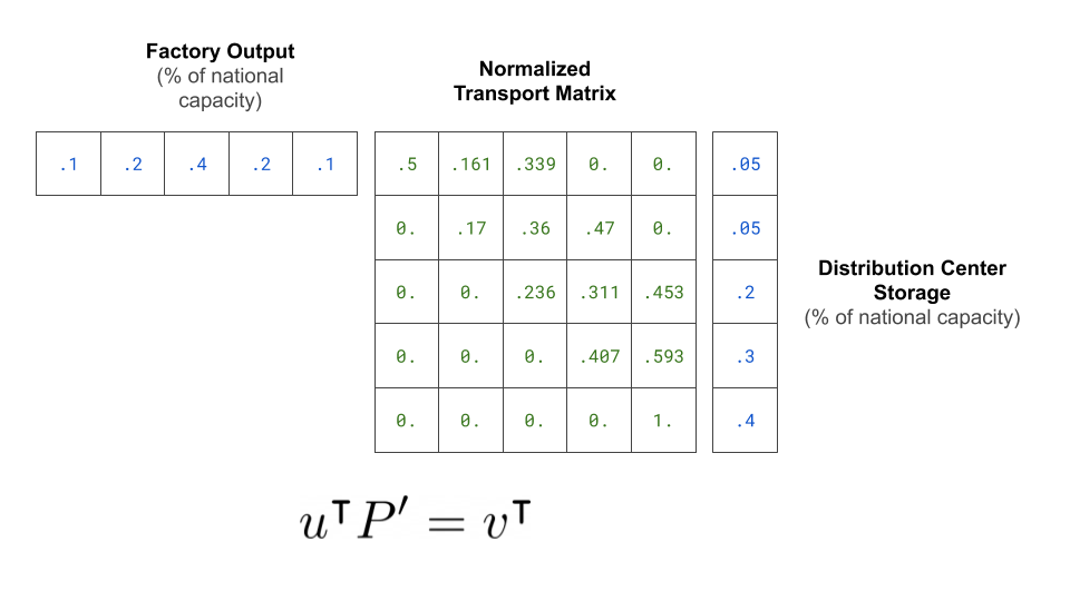
If we rescale our transport matrix such that the rows sum to 1, we can view this rescaled transport matrix, \(P^{\prime}\) as a matrix that acts on our source distribution to produce our target distribution (like transition probabilities in a graph).
$$ P^{\prime}_{ij} = \frac{P_{ij}}{\sum_{j=0}^{M} P_{ij}} $$
$$ v^{\intercal} = {u}^{\intercal} P^{\prime} $$
Algorithms for Computing Optimal Transport
Now, how do we go about discovering the optimal transport matrix?
One solution to our dilemma would be to compute an optimal strategy using linear programming methods. We'd express the cost of transporting a roll of Charmin Ultra Plush from each of the N factories to each of the M distribution centers as a equation to minimize, subject to our linear system of constraints. For Charmin, this solution might be appropriate, but as N and M increase the cost of the linear programming solution increases sharply.
An alternative to linear programming is to use an iterative method to efficiently approximate the exact solution. The Sinkhorn-Knopp algorithm takes as input:
- A cost matrix, \(M\)
- A discrete source distribution, \(u\),
- A discrete target distribution, \(v\)
- A regularization parameter, \(\lambda\)
- An convergence parameter that we use to decide when to stop our iterative algorithm.
Because we're iteratively computing an approximation of the transport matrix, our convergence parameter is simply of how precise the approximation needs to be before we stop iterating.
The regularization term controls the initialization of the proposed transport matrix. A higher regularization term encourages a more uniform initialization of \(P\), while small regularization values encourage a sharper distribution. This means we're not strictly computing the optimal transport matrix – we've added a smoothing term to our global cost.
Sinkhorn Distance
The value the Sinkhorn-Knopp algorithm minimizes is the Sinkhorn distance:
$$ \sum_{\forall i, j}{M_{ij} P_{ij}} + \lambda {P_{ij} \log P_{ij}} $$
For large values of lambda, the term on the right dominates, and we solution we arrive at is more homogeneous – for our Charmin Ultra-Soft example, factories would send some amount of their toilet paper to each of the distribution centers. This could be desirable behavior if you want to prevent single-points of failure in your supply chain. As lambda approaches zero, we are left with only the term on the left – the Wasserstein distance.
You might recognize the term on the right as a negation of an information entropy term, \(-{P_{ij} \log P_{ij}}\). Since we're minimizing this sum, the regularization can be viewed as encouraging higher entropy (more uniformly distributed) transport matrices.
The Sinkhorn-Knopp Algorithm
I've added some inline commentary, but the full Sinkhorn-Knopp algorithm is quite concise – less than 10 functional lines of code. An interactive version of the code in this blog post is also available as a Google colab notebook.
import numpy as np

def sinkhorn_knopp(cost_matrix, source, target, reg, eps):
    # Largest entries of P correspond to
    # movements with lowest cost
    P = np.exp(-cost_matrix / reg)
    P /= transport_matrix.sum()

    # Source corresponds to rows,
    # target corresponds to colums
    source = source.reshape(-1, 1)
    target = target.reshape(1, -1)

    err = 1
    while err > eps:
        # Over time this both the row_ratio and
        # col_ratio should approach vectors of all 1s
        # as our transport matrix approximation improves
        row_ratio = source / P.sum(axis=1, keepdims=True)
        transport_matrix *= row_ratio
        col_ratio = target / P.sum(axis=0, keepdims=True)
        transport_matrix *= col_ratio

        # If we've just normalized our columns to sum
        # to our target distribution, and the sum of
        # our rows is still a good approximation of our
        # source distribution, we've converged!
        err = np.max(np.abs(P.sum(1, keepdims=True) - source))

    min_cost = np.sum(transport_matrix * cost_matrix)
    return transport_matrix, min_cost
The first two lines of the algorithm initialize our transport matrix. Each entry in the matrix is proportional to \(e^{-M_{ij}}\), so as cost increases the corresponding transport matrix entry drops to zero.
P = np.exp(-cost_matrix / reg)
P /= transport_matrix.sum()
The heart of our algorithm simply iteratively normalizes the rows and columns such that they sum to our source and target distributions respectively.
while err > eps:
    row_ratio = source / P.sum(axis=1, keepdims=True)
    transport_matrix *= row_ratio
    col_ratio = target / P.sum(axis=0, keepdims=True)
    transport_matrix *= col_ratio
    err = np.max(np.abs(P.sum(1, keepdims=True) - source))
In practice the Sinkhorn iterations are often translated into the log domain to avoid overflow / underflow.
Sinkhorn-Knopp for Charmin Ultra-Soft
Now we've defined the Sinkhorn-Knopp algorithm, we can plug in the values for our toy Charmin Ultra-Soft distribution problem to find the optimal transport plan given a choice of \(\lambda\).
source_dist = np.array([0.1, 0.2, 0.4, 0.2, 0.1])
target_dist = np.array([0.05, 0.05, 0.2, 0.3, 0.4])

# Cost proportional to distance between bucket idxs
cost_matrix = (
    np.arange(len(source_dist)).reshape(1, -1) -
    np.arange(len(target_dist)).reshape(-1, 1)
)

transport_matrix, min_cost = sinkhorn_knopp(
    cost_matrix,
    source_dist,
    target_dist,
    reg=0.01,
    eps=1e-4
)

# ~ 0.947
print(min_cost)
If we plot our error terms over time, we can see the column sums converge to the value of our source distribution, and the row sums correspondingly converge to the value of our target distribution.
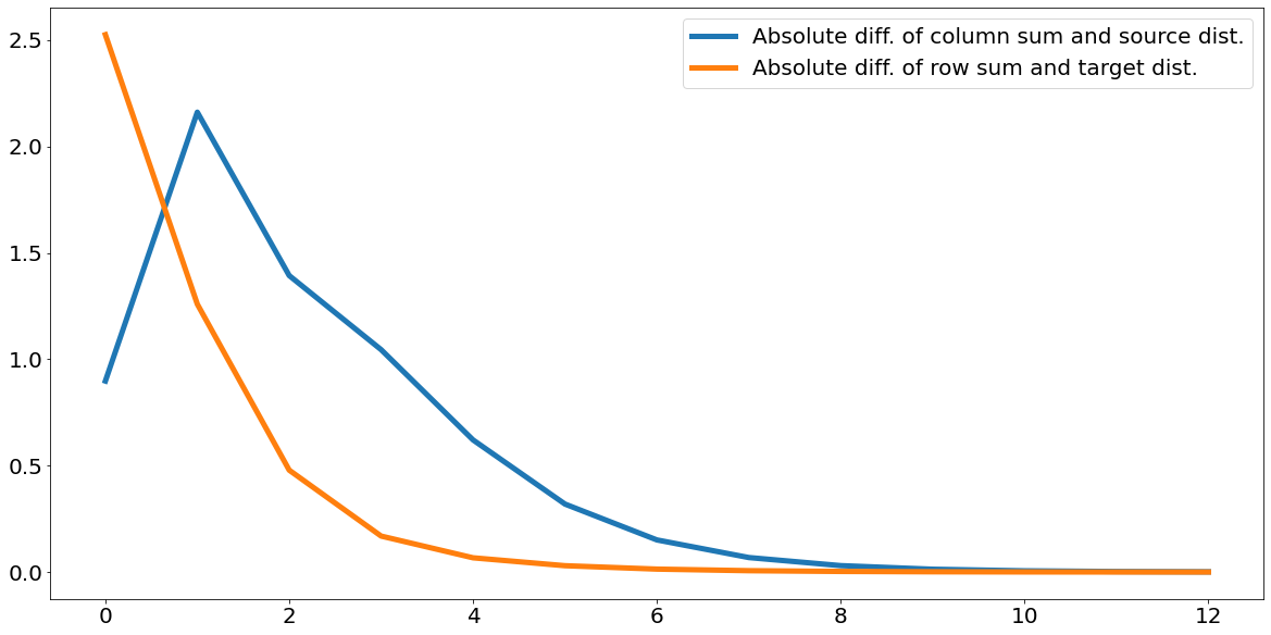
Neat! Simple iterative normalization was sufficient for us to derive an optimal transport plan. Even better, since we can trivially differentiate through the normalization operation, this iterative approximation is a valid building block for inclusion in a neural network trained with SGD.
Differentiable Sorting
Before you celebrate however, let's take a step back. We set off to understand how we could define a differential sorting operation, but so far we've been talking about optimal transport. How do we apply this method to a sorting task?
Well, sorting is quite similar to optimal transport! We can interpret our source distribution as being an unsorted sequence and the target distribution as being the sorted sequence. We just have a few additional constraints.
- We'll assign every entry in the source and target distribution to a value of 1.
- Our source and target distributions must be vectors of the same size.
- Since we want each input to map to 1 and only 1 output, we'll use a small regularization parameter as we want "sharp" output distributions.
To show this in action, let's initialize a random cost matrix and use it to "sort" our input sequence in the order which minimizes global cost.
source_dist = np.array([1, 1, 1, 1, 1])
target_dist = np.array([1, 1, 1, 1, 1])
cost_matrix = np.random.random((5, 5))

transport_matrix, min_cost = sinkhorn_knopp(
    cost_matrix,
    source_dist,
    target_dist,
    reg=0.001,
    eps=1e-4
)

print("Transport matrix", transport_matrix)
print("Min cost", min_cost)
Which outputs:
Transport matrix
 [[0. 0. 0. 1. 0.]
  [0. 1. 0. 0. 0.]
  [1. 0. 0. 0. 0.]
  [0. 0. 1. 0. 0.]
  [0. 0. 0. 0. 1.]]
Min cost
 1.2920057051570364
Source index 0 is mapped to target index 3, source index 1 is mapped to output index 1, and so on. We've repurposed our optimal transport solver for a sorting task by only changing our inputs, and have come full circle to our original motivating problem of differentiable sorting!
Note that a sparse output matrix isn't strictly guaranteed – if our regularization term is too large or our costs are too similar, we may not be able to interpret our transport matrix as a sorting matrix.
Now that we understand the mechanics of differentiable sorting using Sinkhorn iterations, let's jump back to the present and see how this method is applied as part of "Sparse Sinkhorn Attention".
Sinkhorn Transformer
The key contribution in "Sparse Sinkhorn Attention" is the introduction of a differentiable sorting-based method to enable information share between tokens that might be far apart in reading order.
The Sparse Sinkhorn Attention paper first introduces the concept of "SortNet" – a parametric sorting operation.
Sorting our Input Sequence
First, the sequence is partitioned up into \(N_b\) buckets of length \(b\), the bucket size. These are the blocks that we will end up sorting with Sinkhorn iterations. At first, these buckets are purely determined by locality in the sequence. The first \(b\) tokens are placed into bucket 0, the next \(b\) tokens are placed in bucket 1, and so on.
Then, token-wise representations are mean-pooled within each bucket to produce a per-bucket activation we'll refer to as \(X^{\prime}\).
We pass each bucket's representation through a parametric transformation to output a vector of size \(N_b\). The authors select a simple two layer MLP with ReLU activations to perform this transformation.
Now we're back in familiar territory. We can think of the outputs of the MLP as being equivalent to a column vector of transport costs in our Sinkhorn algorithm – the ith entry in the output vectors represents the "cost" to move the contents of that bucket to the ith output location! The ReLU activations ensure that the transport cost is always a positive value (i.e., a valid input to the Sinkhorn algorithm).
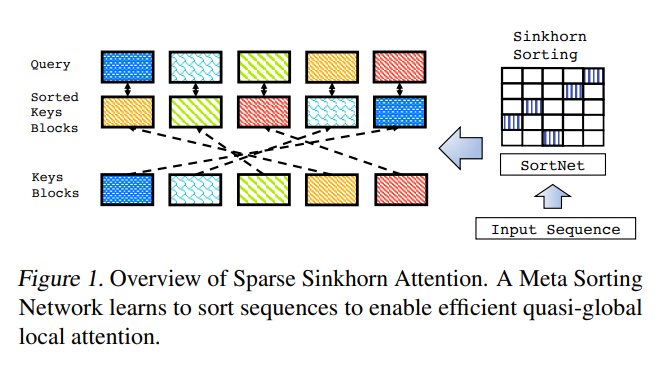
Because we have \(N_b\) buckets, we can concatenate the per-bucket MLP outputs together to form output matrix of shape \((N_b, N_b)\) that the authors refer to as the sorting matrix, or \(M\) – shown in the right hand side of the graphic above – effectively the same \(M\) we discussed prior in our optimal transport example!
We apply the Sinkhorn-Knopp algorithm to our cost matrix M, using vectors of all 1's to represent our source and target distributions, and backpropagate through this operation at training time. Rather than waiting for converge, a fixed number of Sinkhorn iterations (typically between 5-10) is applied. The output of the Sinkhorn-Knopp algorithm is then our sorting matrix.
Once we've computed our sorting matrix, we can apply it to re-order the buckets of our input sequence. Tokens are first grouped into blocks based on locality, we apply the sorting matrix to reorder the blocks, and finally reshape the blocks back into a sequence of tokens. So through the use of the Sinkhorn-Knopp algorithm, we've managed to define a fully-differentiable operation that reorders our input sequence! This entire operation we'll refer to as \(\psi\).
Note that we don't actually need our sorting matrix to be discrete! If our regularization term is small enough, it likely will be, but we're free to increase our regularization term and blend the representations of several buckets to produce each output entry (just like several factories often supplied a single distribution center in our toilet-paper distribution example). Although it's perhaps easier to visualize the variant of this approach where a discrete sorting operation is used, the soft-variant is perfectly valid. In fact, the authors found that the soft version of the sorting operation typically worked better than the hard variant. One reason for this may be that the Sinkhorn algorithm typically requires more iterations to converge for smaller regularization terms.
Using our Sorted Sequence in the Attention Operation
Critically, if there is information from a far-away bucket that happens to be relevant to the bucket of interest, we can re-sort the sequence to expose that information to the current block.
Say that we're concerned with processing the contents of bucket 12. Bucket 3 contains information that would help in the understanding of our current block. If our sorting operation, \(\psi\), resorts the sequence such that bucket 3 is moved to location 12, our current bucket will be allowed to attend to that bucket in the process of producing its next hidden state.
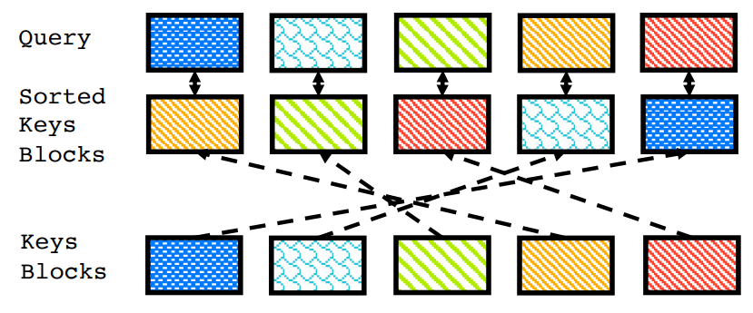
More precisely, the attention weight between query \(i\) and key \(j\) is given by the equation below, that blends the sorted attention term with a standard local attention term.

The sorting operation is also applied to the sequence of values, meaning the output of the full attention operation is given by:
$$ Y = \text{Softmax}(A)\psi(V) $$
Just like typical dense attention, you can reshape your hidden states into heads to sort and attend over N distinct partitions of your hidden state in parallel. A unique sorting matrix can be learned per head.
Applying this method to an auto-regression language modeling objective is quite tricky because of the requirements of causal masking, so I encourage you to refer to the original paper if you're curious how this constraint is satisfied.
SortCut
In the sorting framework we just discussed, each block attends to itself and exactly one other block. This assumes that each block contains information that is useful to exactly one other block in the sequence. In practice, I'd be quite surprised if this assumption held – I'd assume instead that the information contained in a small number of blocks is disproportionately useful to the rest of the sequence. Perhaps to encourage behavior that better aligns with this hypothesis, the authors propose a variant to this sorting methodology that they call "SortCut".
Much of the implementation stays the same, but the manner in which they choose to use the sorted sequence varies. Instead of having the sorting operation match each block up with another block in the sequence, they interpret the sorted buckets as a sort of priority order of long-term information. All of the query terms are allowed to attend to the first \(k\) terms of the sequence, and the rest of the sequence is cut off.
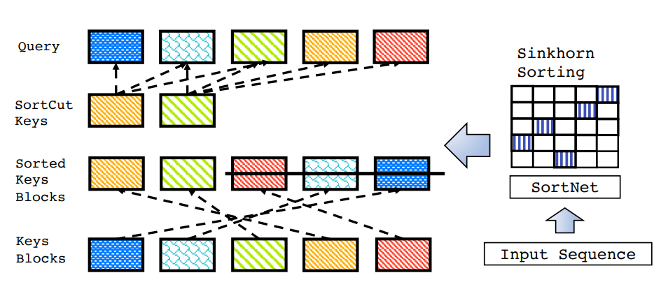
Notably, we don't actually need to compute the sorted keys and values for buckets past the cutoff, allowing us to save a substantial amount of memory at long sequence lengths.
Complexity Analysis
For a sequence of length \(\ell\), runtime complexity of traditional dense attention scales with \(O(\ell^2\)). Because we constrain attention to only be performed within a bucket with a sufficiently small number of items, if we have \(N_B\) buckets with \(b\) tokens each, the runtime complexity of Sinkhorn attention is \(O(\ell b + N_B^2)\). The SortCut has similar characteristics, with a runtime complexity of \(O(\ell b k + N_B^2)\), where k is the truncated number of buckets.
Memory complexity is also improved over dense attentions. By preventing storage of the full \(O(\ell^2)\) attention matrix and attending only over buckets, memory complexity is reduced by a factor of \(N_B\) when compared to dense attention (a complexity similar to local attention). Even better, SortCut only requires storing \(O(\ell b k + N_B^2)\) attention weights. When \(b\) is sufficiently low, this means its memory complexity is effectively linear with sequence length.
Empirical Results
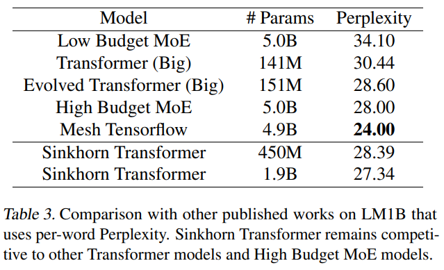
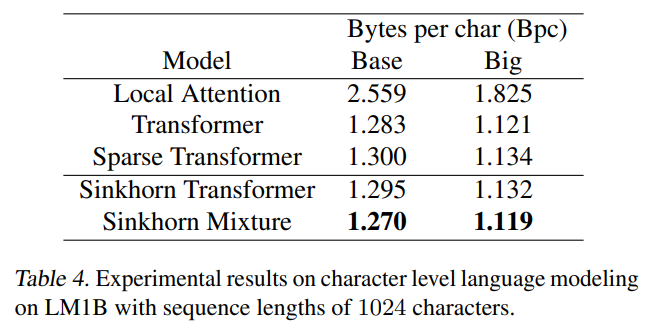
The Sinkhorn transformer shows strong performance on a token and char level language modeling tasks on LM1B.
On a word-level language modeling benchmark, the Sinkhorn transformer produced perplexities competitive with a larger mixture of experts model on LM1B.
On character level tasks, the Sinkhorn transformer slightly outperformed the block-sparse transformer at similar parameter budgets.
The authors also achieve competitive results on a pixel-wise image generation task (CIFAR-10).
I appreciate that they abstained from reporting scores on standard language modeling benchmarks like enwik8, text8, and PTB, as recent twitter commentary suggests that small dataset size limits the utility of those benchmarks and heavy regularization is necessary to achieve competitive perplexities.
Further Reading and Closing Thoughts
- An open source implementation of the Sinkhorn Transformer (with some Reformer and Routing inspired bells and whistles) is available thanks to the work of Philip Wang. Also included in his experiments are versions of the Sinkhorn Transformer that replace the Sinkhorn iterations with a simple softmax operation while still achieving competitive performance – I'm eager to see where this line of research leads!
- Michiel Stock's "Optimal Transport" blog post was tremendously helpful in developing my own understanding of the Sinkhorn algorithm, and I'd highly recommend it to those who were unfamiliar with optimal transport prior to this blog post.
- Gabriel Peyré and Marco Cuturi have compiled a 200 page report on optimal transport and it's variants. If you're interested in the theory behind the Sinkhorn algorithm, there's a wealth of knowledge available in their work "Computational Optimal Transport".
Thanks go out to @lucidrains and @arankomatsuzaki for discussion related to the Sinkhorn transformer and variants.
Feedback (constructive or otherwise) is always welcome – feel free to reach out directly to madison@indico.io.


