A Survey of Long-Term Context in Transformers

It's no secret that multi-head self-attention is expensive -- the \(O(n²)\) complexity with respect to sequence length means allowing vanilla transformers to attend to long sequences quickly becomes intractable. Over the past two years the NLP community has developed a veritable zoo of methods to combat this problematic complexity, but in this post we'll focus on a dozen promising approaches. You can click on any of the links below to jump directly to that section of the post.

1. Sparse Transformers
2. Adaptive Span Transformers
3. Transformer-XL
4. Compressive Transformers
5. Reformer
6. Routing Transformer
7. Sinkhorn Transformer
8. Linformer
9. Efficient Attention: Attention with Linear Complexities
10. Transformers are RNNs
11. ETC
12. Longformer

Time and Memory Complexity of Dense Multi-Head Attention

Multi-head attention scales poorly with sequence length for two reasons.  The first is that the number of FLOPs required to compute the attention matrix scales with the square of the sequence length, resulting in a computational complexity of \(O(hdn²)\) for a self-attention operation on a single sequence, where \(h\) is the number of attention heads, and \(d\) is the dimension of keys and queries, and \(n\) is the length of our sequence.  

Equally problematically, the memory complexity of the dot-product self-attention operation also scales with the square of the sequence length.  The memory complexity to compute the attention matrix is \(O(hdn + hn²)\) – the first term being the memory required to store keys and queries, and the second term referring to the scalar attention values produced by each head.

Let's substitute in some concrete numbers from BERT-Base to get a sense for what terms dominate.  BERT-Base uses a sequence length of 512, a hidden size of 768, and 12 heads, which means that each head has dimension 64 (768 / 12).  In this setting, 393216 floats (~1.5MB) (12 heads * 64 head size * 512 sequence length) are required to store the keys and values, while the memory required to store the scalar attention values for all head works out to 3,145,728 floats (12 * 512 * 512) or ~12MB of device memory – nearly 10 times as much memory as storing the keys at a mere 512 token context size.

Since activations must be cached during training to allow for gradient computation (barring the use of activation re-computation strategies like gradient checkpointing), storing just these attention matrices for all 12 layers of BERT base requires about ~150MB of memory per example.  At sequence length 1024 this becomes ~600MB, and at sequence length 2048 we're already up to ~2.4GB of memory per example for the attention matrices alone. This means smaller batch sizes and poorer parallelism at training time, further hindering our ability to train models that leverage long context lengths.

Sparse Transformers

"Generating Long Sequences with Sparse Transformers" by Rewon Child, Scott Gray, Alec Radford, and Ilya Sutskever addresses the problematic \(O(n²)\) term in the time and memory complexity of self-attention via a factorization approach.

Factorized Attention

In a typical self-attention operation, each term in the input sequence attends to all other terms in the input sequence, resulting in an attention pattern shown below:

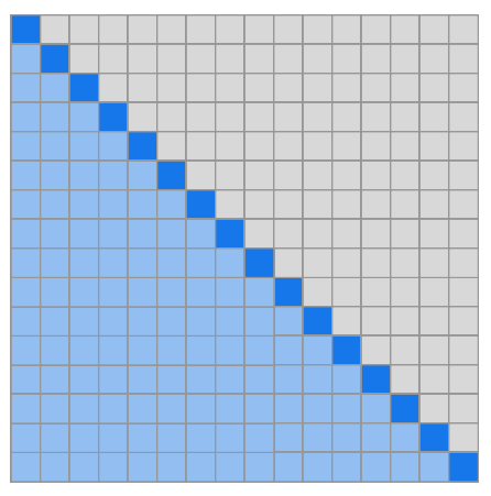
The benefit of typical self-attention is that this high connectivity allows ease of information flow between tokens – only a single layer is necessary to aggregate information from any two tokens.  But if we relax this constraint, and ensure only that information can flow between any two tokens after two layers, we can dramatically reduce our complexity with respect to sequence length. The Sparse Transformer achieves this goal by writing custom kernels that leverage fixed attention patterns.

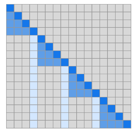
Half of the heads attend only to terms in a short, local context, while the other half attend to predesignated indices spread evenly throughout the sequence.  

By routing information through these aggregation indices the network is still able to pass information from distant tokens and make use of long-term context, while reducing time and memory complexities to \(O(n\sqrt n)\). Importantly, it only requires two layers for any token to incorporate information from any other token.

Empirical Results

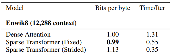
Importantly, the factorized attention structure doesn't seem to negatively impact language modeling performance, leading to bits per character that were (surprisingly) marginally better than dense attention on enwiki8 and allowing efficient attention over context sizes up to 12,228 tokens.

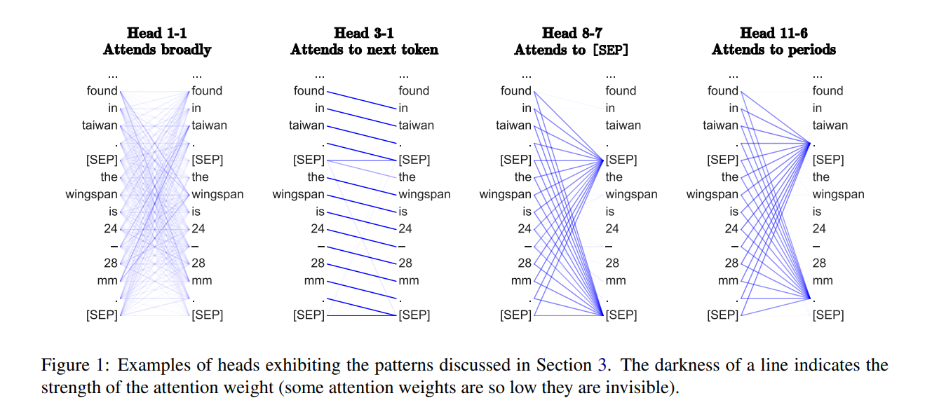
It's conceivable that the Sparse Transformer attention structure works in part because these attention patterns aren't all that dissimilar from real learned dense attention patterns.  In "What Does BERT Look At? An Analysis of BERT’s Attention" by Kevin Clark, Urvashi Khandelwal, Omer Levy, and Christopher D. Manning the authors probe the patterns learned by dense attention in an effort to gain intuition for what functions attention performs in transformer models. They find heads that attend to the token immediately previous (similar to the local attention pattern in sparse attention) as well as heads that attend to specific aggregation tokens like [SEP] and periods. So perhaps the inductive biases encoded in the Sparse Transformers attention patterns are useful rather than detrimental.

To employ the fixed attention kernels in your own projects, check out OpenAI's blocksparse library and the accompanying examples the authors have released as open source.

Adaptive Span Transformers

Sainbayar Sukhbaatar, Edouard Grave, Piotr Bojanowski, and Armand Joulin take a different approach to the complexity problem in their work "Adaptive Attention Span in Transformers".  They make a similar observations to the authors of "What Does Bert Look At?" and note that while dense attention allows each head to attend over the full context, many attention heads specialize to only consider local context while others consider the entire available sequence.  They propose leveraging this observation by using a variant of self-attention that allows the model to select it's context size.

Adaptive Masking

The Adaptive Span Transformer accomplishes this by masking the sequence such that the contribution of tokens outside of a learned, per-head context fall off quickly to zero.  The mask (\(M\)) is multiplied with the logits of the softmax operation to zero out certain tokens' contributions to the current hidden state, \(x\), and a hyperparameter \(R\) controls the minimum span size.

$$ M = min(max(\frac{1}{R}(R + z - x), 0), 1)$$

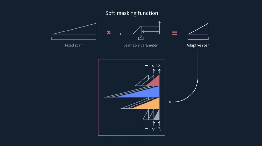
An \(\ell_1\) penalty is applied to the learned z values in order to encourage the model to only use additional context where beneficial.  

Attention Introspection and Empirical Results

With these constraints, most heads elect to focus on <100 characters of context, with only a few select heads (primarily in the later layers of the network) opting to pay the \(\ell_1\) penalty in order to attend to a context of >1000 characters.

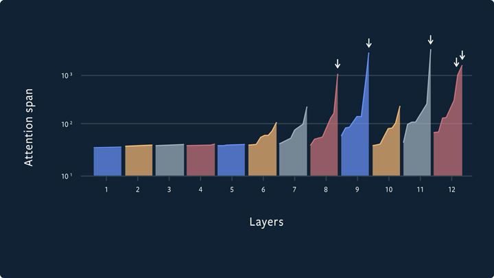
Along with clever caching, this penalty on long term context allows the adaptive-span transformer to use attention spans of up to 8k characters for select heads while still keeping the overall computational cost of the model cheap. In addition, performance on benchmarks remains high, reaching 0.98 bits per character on enwiki8 and 1.07 bits per character on the text8 dataset.

However, the variable span sizes aren't ideal in terms of ease of parallelism where we typically want dense, uniformly sized matrices for best performance. Although this method allows a dramatic reduction in the number of FLOPS necessary to compute the forward pass at prediction time, the authors only provide vague performance estimates, stating that the adaptive span implementation allowed for processing context lengths up to 8192 tokens at similar rates to a fixed context size model with 2048 tokens of context.  

Facebook AI Research has also open sourced their work – code and pretrained models are available at github.com/facebookresearch/adaptive-spans.

Transformer-XL

Rather than attempting to make the dense attention operation cheaper,
Zihang Dai, Zhilin Yang, Yiming Yang, Jaime Carbonell, Quoc V. Le, and Ruslan Salakhutdinov opted to take inspiration from RNNs and introduce a recurrence mechanism in addition to the self-attention mechanism in transformers.  Their work "Transformer-XL: Attentive Language Models Beyond a Fixed-Length Context", introduces two novel concepts – a component that feeds the hidden states of previous "segments" as inputs to current segments layers, and a relative position encoding scheme to facilitate this strategy.

Segment Recurrence

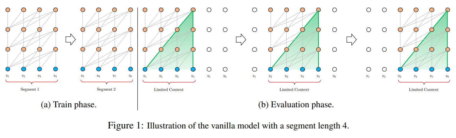
With a standard transformer that has fixed context size, handling long inputs requires splitting the input up into chunks (segments) and processing each individually. However, this approach has the limitation that information from prior segments cannot flow to the current token.  This independence is somewhat beneficial in that it allows for the segments to be batch processed efficiently, but if your goal is long-term coherence this is a major limiting factor.

Transformer-XL overcomes this limitation by enforcing that the segments be processed in series.  After the first segment, tokens in subsequent tokens will always have an immediate context size of 512 tokens, as the previous segments activation are passed as context to subsequent segment's attention operations.  This means that information from \(N\) context size * \(L\) layers away can be propagated to a given token.  Assuming a context size of 640 and a model with 16 layers, the Transformer-XL can theoretically incorporate signal from up to 10,240 tokens away.

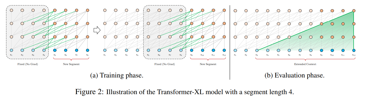
In order to avoid having to store activations from all previous segments, the author's stop gradients from flowing through to previous segments.

Incorporating Relative Position

Transformer-XL also introduces a novel position encoding scheme they deem "relative position encodings".  Rather than simply treating the networks inputs as a sum of content and absolute position embeddings, each layers attention operation is broken up into a portion that attends based on content and a portion that attends based on relative position – for the 512th token in a chunk to attend to the 511th, the embedding corresponding to relative position -1 is used.

To make the use of relative position encodings tractable, they break up the operation that produces attention weights from the keys and queries. For a typical dense-attention operation, the pre-softmax attention weights can be decomposed as follows:

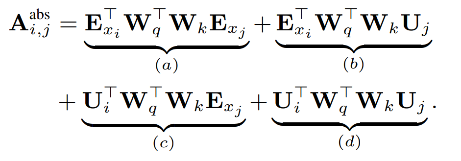
In the equation above, \(E_{x_i}\) is the content-based embedding of token at location \(i\), and \(U_j\) is the position embedding for token \(j\).

\(a)\) relates the query's content with the key's content

\(b)\) relates the query's content with the key's position

\(c)\) relates the query's position with the key's content

\(d)\) relates the query's position with the key's position

When using relative position embeddings, the author's modify the equation as follows:

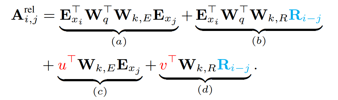
In \(b)\) and \(d)\), \(U_j\) has been replaced with it's relative position counterpart, \(R_{i-j}\).

For the terms that included the query's position, we substitute the matrix \(U_i\) for two new learned parameters, \(u\) and \(v\).  These vectors can now be interpreted as two biases that don't depend on the specifics of the query – \(c\) encourages attends to some terms more than others, and \(d\) encourages attending to some relative positions more than others.  This substitution is motivated by the relative position of the query with respect to itself remaining constant.

Attention Introspection and Empirical Results

For the Transformer-XL model to make use of such long term context, at least one head from each layer would have to make use the full context of its attention span.  A plot of average attention weights show that there are heads from every layer that attend broadly to prior positions.

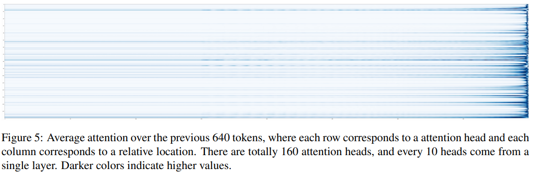
In addition the Transformer-XL paper measures the impact of effective context length on perplexity and finds that increasing context length leads to better perplexity scores up to a context length of ~900 tokens – further evidence that the recurrence mechanism is useful in practice and not merely in theory.

See Kimi Young's github for source code or check out the HuggingFace implementation to start using Transformer-XL for your own side project.

Compressive Transformers

The next model on our list, the Compressive Transformer, builds off of Transformer-XL architecture and extends their methodology with a compressive loss to incorporate even longer sequence lengths. In the work "Compressive Transformers for Long-Range Sequence Modelling", Jack W. Rae, Anna Potapenko, Siddhant M. Jayakumar, and Timothy P. Lillicrap from DeepMind detail a model architecture capable of attending to sequences as long as full length books.

Compressive Transformer Attention

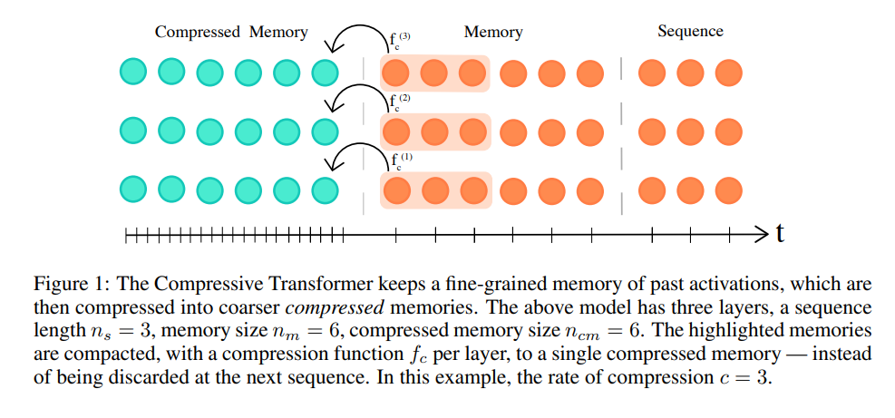
Following Transformer-XL's suit, the sequence can attend to a set of stored activations from previous segments. In addition, in the same multi-head attention operation, tokens in current segment can attend to a second set of states stored in "compressed memory".  

At each time step, the oldest compressed memories are discarded and the compressed memory is shifted back a single index.  Then, the oldest \(n\) states from the normal memory segment undergo compression and are shifted into the newly open slot in the compressed memory.

A gif from the DeepMind blog illustrates this process nicely:

The DeepMind team tried a variety of compressive operations (including baselines like mean pooling, max pooling, and learned convolutions), but settled on training a secondary network to reconstruct the content-based attention matrix of the memory being compressed.  

In other words, they learn a function, \(f_c\), that compresses the \(n\) oldest memory states to a single compresses memory state, by minimize the difference between attention over the compressed memory (\(C_{-1} = f_c(M_old)\)) and attention over the states in normal memory being compressed:

$${\sigma((XW^Q)(M_{0..n} W^K))(M_{0..n} W^V)} - {\sigma((XW^Q)(C_{-1}W^K))(C_{-1}W^V)}$$

Rather than training this compressive operation jointly with the main language model, they opt to update the compressive network in a separate optimization loop, as making the attention states easily compressible is counter-productive to reducing the language modeling loss.

Empirical Results

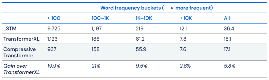
For their experiments, they use a compressed memory size of 512, a memory size of 512, a window size of 512, and a compression rate of 2 – meaning the 2 oldest memory states are compressed to a single state during the compression step. Using these settings they achieve a new state of the art test perplexity of 17.1 on WikiText-103.

As the gains from exploiting longer sequence lengths are typically long tail, they look specifically at perplexity bucketed by token rarity and note that gains are especially notable on the rarest tokens:

Although their source code is not yet public, DeepMind has open sourced PG-19, the dataset they developed while working on the Compressive Transformer. PG-19 is a Project Gutenberg derivative intended to further research into long-term attention.

Reformer

Next up we have a work by Nikita Kitaev, Łukasz Kaiser, Anselm Levskaya entitled "Reformer: The Efficient Transformer". The Reformer takes a different tack at increasing sequence length – rather than introducing recurrence mechanisms or a compressive memory, they opt to narrow the scope of each token's attention by using locality sensitive hashing techniques.  

Locality sensitive hashing is a family of methods that map high dimensional vectors to a set of discrete values (buckets / clusters). It's most commonly used for as a method for approximate nearest neighbor search.

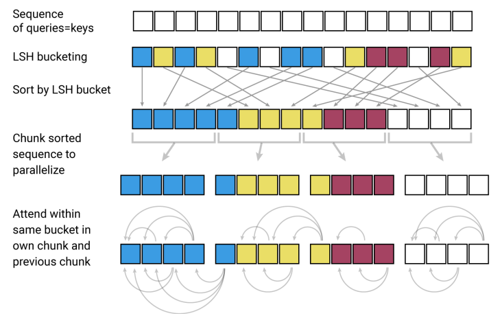
The Reformer authors use a single projection for both the keys and queries of the attention operation, and use a random rotation-based locality sensitive hashing method to group the shared keys / queries into buckets of at most a few hundred tokens. An illustration of the hashing method is below:

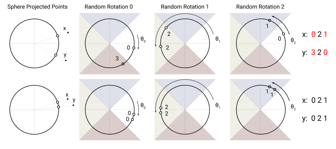
They compute attention matrices within each bucket and then take a weighted sum of the corresponding values.  Because they attend only to elements within a given bucket, this can reduce the overall complexity of the attention operation from \(O(n^2)\) to \(O(n \log{n})\) if bucket size is selected appropriately. Because the bucketing process is stochastic and based on random rotations, they compute several hashes to ensure that tokens which have similar shared key-query embeddings end up in the same bucket with high probability.

They additional employ techniques introduced in "The Reversible Residual Network: Backpropagation Without Storing Activations" to keep train-time memory consumption under control. Reversible residual layers use clever architectural structure to allow the easy re-construction of layer inputs from layer outputs, and trade extra computation for a memory complexity that is constant in network depth.

With the locality sensitive hashing trick to reduce computational cost, and the reversible residuals to reduce memory consumption, the Reformer architecture is able to process sequences of up to 64,000 tokens long on a single accelerator.

Although the reported score of 1.05 bits per character on enwiki-8 lags behind some of the other models we've looked at in the course of this blog post, the Reformer is a refreshingly unique take on a mechanism to incorporate long term context and I'm looking forward to seeing how the approach scales up.

If you're interested in exploring Reformer architecture in more detail, take a look at my recent blog post "A Deep Dive into the Reformer" on the subject.  An open source implementation of the Reformer is available as an example in the google/jax Github repository.  A PyTorch version maintained by Phil Wang is also available.

Routing Transformer

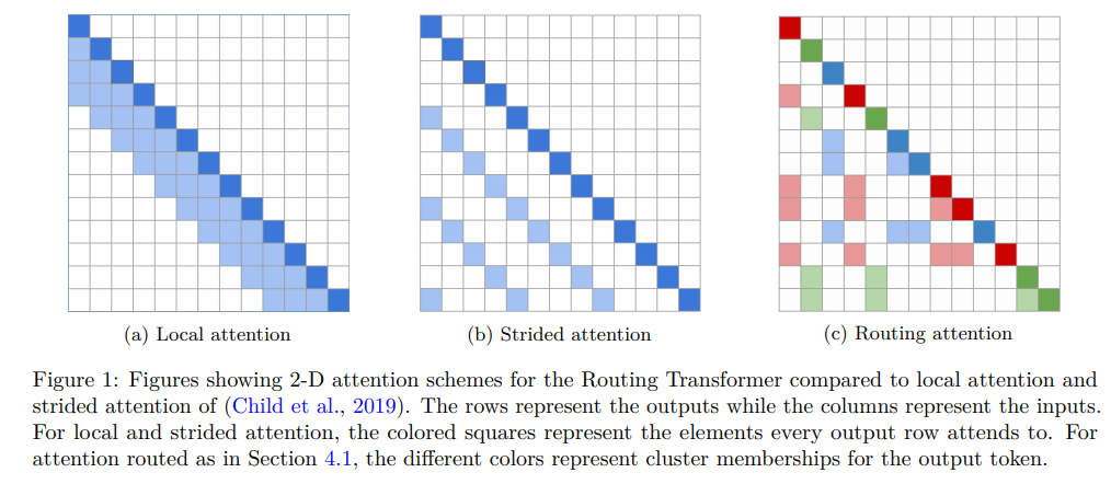
A second paper submitted to ICLR 2020, "Efficient Content-Based Sparse Attention with Routing Transformers" by Aurko Roy, Mohammad Taghi Saffar, David Grangier, and Ashish Vaswani shares some similarities with the aforementioned Reformer. They frame the problem as one of clustering, and aim to learn to select sparse clusters of tokens, \(S_i\), as a function of the content, \(x\).

The author's illustrate their approach in the diagram below.  Rather than solely attending to local elements  or every nth element to increase sparsity, they learn clusters (denoted by color in figure \(c)\) within which to attend. Importantly these clusters are a function of the content of each key and query, not just their absolute or relative positions.

Routing Attention

After ensuring each key and query vector has unit magnitude, they project key and query values using a shared matrix of random orthogonal weights of shape \((D_k, D_k)\), where \(D_k\) is the hidden dimension of the keys and queries.

$$ R = \begin{bmatrix} Q, K \end{bmatrix} \begin{bmatrix} W_R \\ W_R \end{bmatrix}$$

The vectors in R are then grouped into k-clusters according to a set of k-means centroids into clusters, \(C\).  The k-means centroids are learned separate from the gradient descent process, using one application of the k-means update rule per batch.

Within a given cluster, \(C_i\), they compute a new set of contextual embeddings using a typical weighted sum of values, where each attention value, \(A_i\) is computed using typical dot-product self attention.

$$ X_i^{\prime} = \sum_{j \in C_k}{A_{ij}V_j} $$

Because attention patterns in dense attention are often dominated by a few key elements, and because the cluster assignment process should group keys and queries with high attention weights into the same cluster, the authors argue that this preserves the key information that would have informed \(X_i^{\prime}\) had an expensive dense operation been applied.

Finally, they choose a number of clusters close to \(\sqrt{n}\), so that the overall complexity of their sparse content-based attention mechanism becomes \(O(n\sqrt{n})\).  To make the whole process easily parallelizable and deal with matrices of uniform size, the authors use the top-k terms closest to a each centroid in place of the true k-means clusters assignments.

In addition to the content-based routing attention, the Routing Transformer also performs local attention over a context window of size 256.

Empirical Results

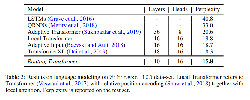
The Routing Transformer's gains in computational efficiency also lead to perplexity gains on Wikitext-103, a word-level language modeling benchmark, where they edge out the Transformer-XL model described previously by a significant margin.

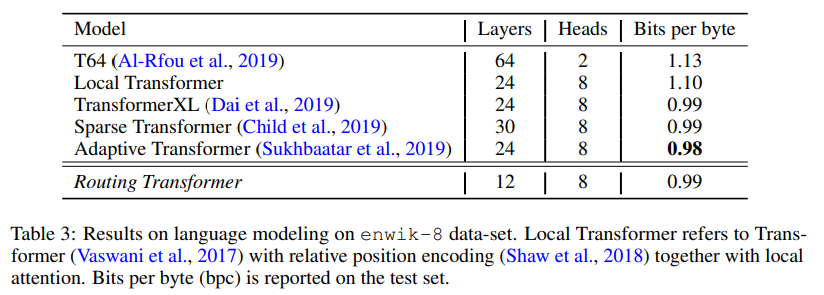
On enwiki-8, the Routing Transformer also performs quite well, although their results lag marginally behind the Adaptive Span Transformer.

I originally couldn't find an implementation of the Routing Transformer, but Aurko Roy was kind enough to point me to a zip of their source that was released as part of the ICLR review process.

Sinkhorn Transformer

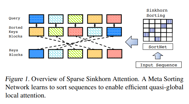
Rather than clustering, the authors of the "Sparse Sinkhorn Attention" (Yi Tay, Dara Bahri, Liu Yang, Donald Metzler, Da-Cheng Juan) draw inspiration from differentiable sorting and the optimal transport domain. I've previously covered this paper in detail in my blog post "Optimal Transport and the Sinkhorn Transformer" but a shorter summary is included below.

Background on Optimal Transport

Optimal transport aims to learn a mapping (the transport matrix) between two distributions. Its often applied to problems of logistics, like learning the optimal distribution strategy between a set of factories and a set of warehouses. In discrete cases like the factory and warehouse problem, there's a fixed cost assigned with moving goods between each factory / distribution center pair (illustrated below).

The optimal transport problem aims to find the transport matrix that minimizes the global cost – in our example, given by the sum over all local pair costs multiplied by the amount of material transported between each pair.

The transport matrix that is learned is constrained to have it's rows sum to the entries of one distribution and it's columns sum to the entries of the second.

One could find solutions to the optimal transport problem via linear programming, but the linear programming solution both scales poorly with the number of entries in our matrix and is an ill fit for inclusion in a neural network. To apply the concept of optimal transport to long-term context in the attention operation in a transformer, we look to the "Sinkhorn-Knopp" algorithm – this particular paper's namesake.  After some careful initialization of our transport matrix using a function of our cost matrix, the Sinkhorn-Knopp algorithm iteratively ensures the rows and columns sum to the desired values. After sufficient iterations, the sums of the rows and the columns converge to the expect values and we have our solution.

At this point you may be wondering what this has to do with long-term context.  If you squint your eyes hard enough, the transport map looks similar to the attention weight matrix!  Additionally, because this Sinkhorn-Knopp algorithm only involves iterative normalization, we can differentiate through it!

Model Architecture

To apply this in practice, an input sequence is divided up into a set of discrete chunks. A representation is computed for each chunk by mean-pooling the token representations contained within. After mean pooling, bucket representations are passed through a small 2-layer MLP that produces an output vector with dimensionality equal to the number of buckets (\(N_B\)).  

We can think of this output vector as being equivalent to a column vector of transport costs described in the logistics problem above!  Since this operation is performed for each bucket, we have a \((N_B, N_B)\) matrix that corresponds to our cost matrix in a transport problem.

From there, we can apply the Sinkhorn-Knopp algorithm to compute how information should be routed between buckets (our transport matrix). For each source bucket, we compute a weighted sum of token representations from the buckets with non-zero entries in the transport matrix, and allow the tokens within the source bucket to attend only to this weighted sum of token representations (in addition to attending to tokens within their own bucket).

A rough visual illustration of this process is outlined below, for the case where the transport matrix is binary (each source bucket routes information to a single target bucket, and each target bucket receives information from a single source bucket).  Although this makes for a clean visual and allows us to think about this process as a sort of sorting operation, the authors achieved the best results when the entries of the transport matrix column were spread out over multiple rows (corresponding to a weighted sum of the token representations of several target buckets).

The authors also propose a variant of this algorithm called SortCut – a description of which I've included as part of the blog post that dives deeper into the details of the Sinkhorn Transformer.

Complexity Analysis

Because we constrain attention to only be performed within a bucket with a sufficiently small number of items, if we have \(N_B\) buckets with \(b\) tokens each, the runtime complexity of Sinkhorn attention is \(O(\ell b + N_B^2)\), where \(\ell\) represents sequence length.

Memory complexity is also improved over dense attentions.  By preventing storage of the full \(O(\ell^2)\) attention matrix and attending only over buckets, memory complexity is reduced by a factor of \(N_B\) when compared to dense attention (a complexity similar to local attention).

Empirical Results

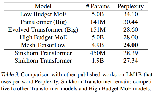
The Sinkhorn Transformer shows strong performance on a token and char level language modeling tasks on LM1B.

On a word-level language modeling benchmark, the Sinkhorn transformer produced perplexities competitive with a larger mixture of experts model on LM1B.

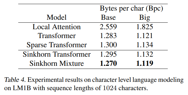
On character level tasks, the Sinkhorn transformer slightly outperformed the block-sparse transformer at similar parameter budgets.

Linformer

The authors of "Linformer: Self-Attention with Linear Complexity" (Sinong Wang, Belinda Z. Li, Madian Khabsa, Han Fang, Hao Ma) take a refreshingly simple approach to dealing with self-attention's quadratic complexity.  The key idea of the Linformer paper is to approximate the attention matrix with a lower rank matrix with size independent of the sequence length.

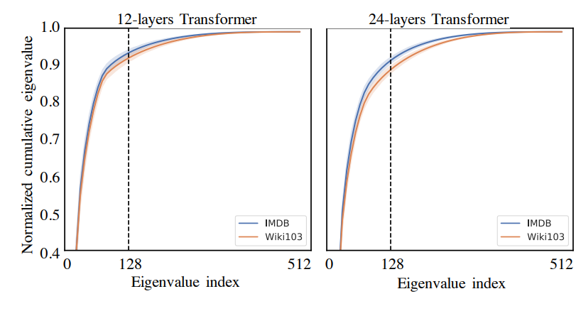
They argue that the effect of multiplying the value matrix by the attention matrix can be approximated well by multiplication with a matrix with fewer columns.  Visualizations of attention weights do generally show that attention weights are dominated by a few key entries (rather than being diffuse attention over the whole sequence), which provides us with some intuition to back up this assertion. If intuition isn't sufficient, however, they provide some SVD visuals that backup their assertion, and demonstrate that >90% of the variation in the attention weight matrix can be explain by the first 128 of 512 eigenvalues.

If you're still not satisfied with the SVD visualizations, they give equations which describe the error-bounds of approximation of the lower rank matrix that replaces the full attention matrix that you can find in the full paper.

Model Architecture

The core model architecture contribution of the Linformer is a set of two projection matrices that function rather atypically from typical projections.

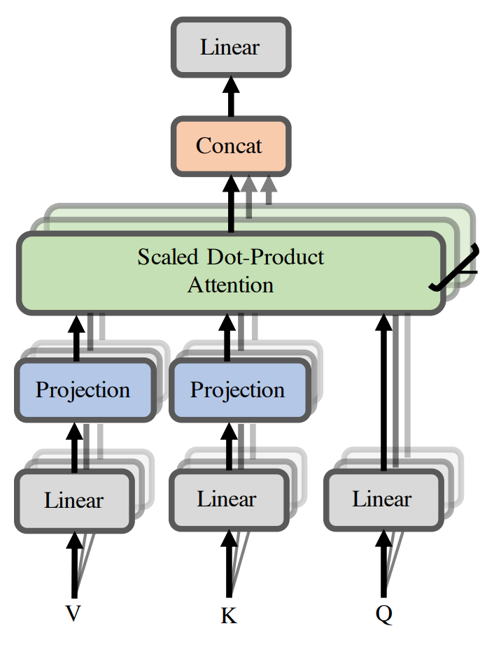
Rather than projecting down the sequence length \(n\) by hidden dim \(d\) matrices down to shape \((n, k\)) and reducing the size of the hidden dimension, they instead project down the sequence length dimension to output a matrix of activations of shape \((k, d)\) for both the keys and values matrices (represented by the blue projections in the diagram below). The query is handled as in vanilla self-attention.

Next, the queries \((n, d)\) and projected keys \((k, d)\) are multiplied together to produce a \((n, k)\) agreement matrix.

Finally, this \((n, k)\) agreement matrix is multiplied with the \((k, d)\) down-projected value matrix to produce an output of shape \((n, d)\) just like in vanilla self-attention.

The down-projection matrices can be viewed rather as producing a set of pseudo-tokens that summarize the sequence – each of \(k\) pseudo-tokens indicates how highly a given filter activate on average when dotted with the full sequence of corresponding representations.

Computational Complexity

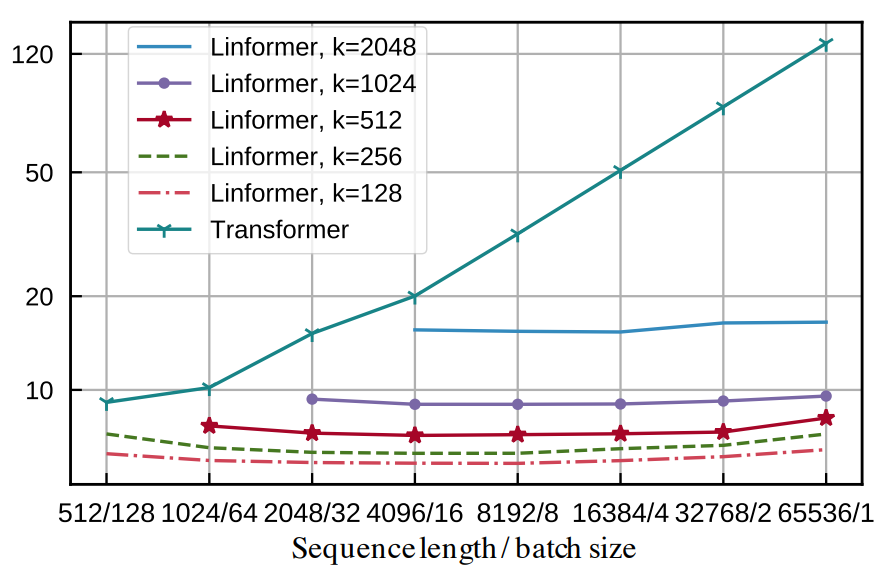
Because d is a fixed-size matrix that does not dependent on sequence length, the computational complexity of this modified transformer operation is in fact \(O(n)\) with respect to sequence length. Similarly, because our matrix of attention weights is shape \((n, k)\) rather than \((n, n)\), the memory complexity of the Linformer is also constant with sequence length.  Empirical data back up the theoretical complexities, with clear evidence that the runtime of the Linformer scales only linearly with sequence length.

Experimental Results

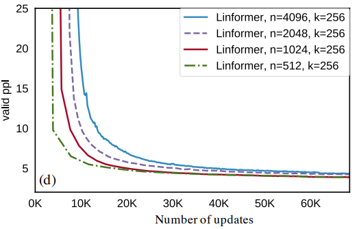
The perplexity of the Linformer manages to stay within a stone's throw of standard transformer perplexities when evaluated on a masked language modeling task on the BooksCorpus and English Wikipedia datasets.

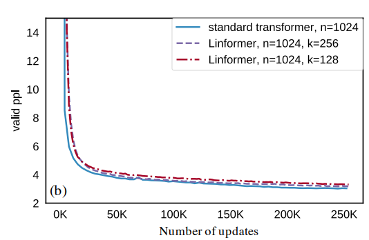
Perplexities tend to increase slightly as sequence length increases – likely because unlike the Sinkhorn Transformer and Routing Transformer, local attention is not included alongside the linear attention mechanism.

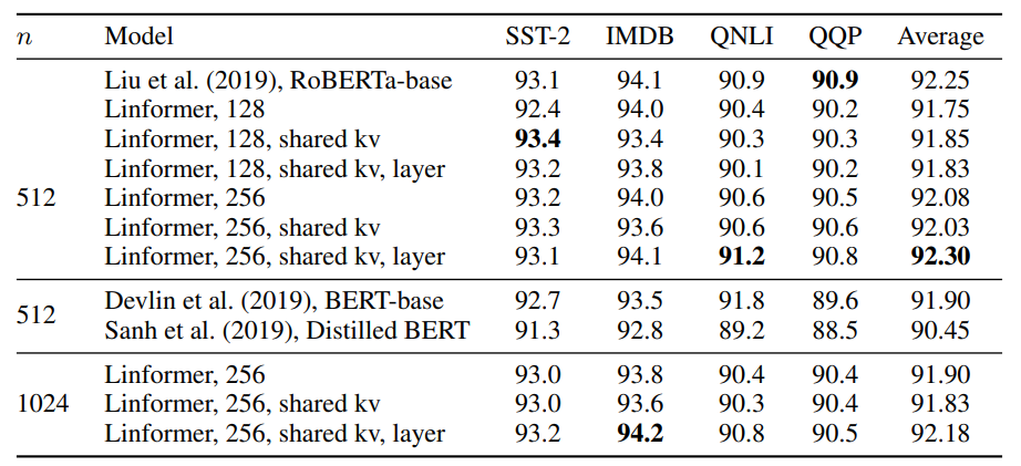
When applied to downstream benchmarks in the form of sentiment and NLI tasks, the Linformer with a matches or slight baseline RoBERTa-base model despite being 30% more runtime efficient and 50% more memory efficient with sequence length \(n\)=512 and projected dimension \(k\)=256.

An unofficial implementation of the linformer is available at https://github.com/tatp22/linformer-pytorch

Similar ideas are explored for the problem of modeling protein sequence in the work "Masked Language Modeling for Proteins via Linearly Scalable Long-Context Transformers" by Krzysztof Choromanski, Valerii Likhosherstov, David Dohan, Xingyou Song, Jared Davis, Tamas Sarlos, David Belanger, Lucy Colwell, and Adrian Weller.

Efficient Attention: Attention with Linear Complexities

The next paper on our list, "Efficient Attention: Attention with Linear Complexities" by Zhuoran Shen, Mingyuan Zhang, Haiyu Zhao, Shuai Yi, and Hongsheng Li, was first posted to arXiv in 2018 but received it's most recent update in Jan. 2020. Their method relies on the observation about the associativity of matrix multiplication.

Self-attention is typically implemented as:
$$ \text{softmax}(QK^{T})V $$

When multiplying two matrices of shape \((a, b)\) and \((b, c)\), we require \( a * b * c\) multiplications.  Disregarding the batch and head dimensions of multi-head attention for purposes of simplicity, this means the multiplication between Q and K would require \(n * d * n\) multiplications to produce a matrix of shape \((n, n)\).  Then we'd perform a matrix multiplication with \(V\) for another \(n * n * d\) multiplications.

If we ignore the softmax normalization for a moment and assume our attention operation is purely a matter of 2 sequential matrix multiplications, because matrix multiplication obeys the associative property we could produce the same output by reordering our matrix multiplications:

$$ (QK^{T})V = Q(K^{T}V) $$

In the latter formulation, we need only \((d * n * d)\) floating point multiplications to multiply our keys and values to produce a \((d, d)\) matrix, and an additional \((d * n * d)\) multiplications to multiply our query with the result of the key and value multiplication.

This gives us a way to incorporate some notion of global context in a manner that is linear with sequence length.  The author's illustrate this change in the diagram below:

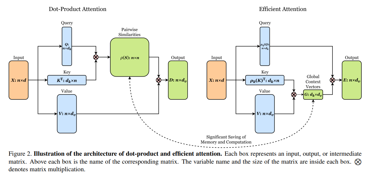
This change requires building up some new intuition about the role of the query, key and value tensors.  We can continue to view the value tensors similarly to before – they represent some information it may be valuable for other tokens in the sequence to attend to.   The keys can be viewed as \(k\) "channels" for that information to be placed in. The "global context vectors" matrix represents a summary of the value information present in each key channel summed over the entire sequence.  And finally, the query vectors select which "channels" are most useful for them to query information from.  The entire efficient attention operation is \(O(n)\) in memory and computational complexity.

To return to problem of the pesky softmax operation that prevents equivalence between these two operations, the authors argue that independently applying a softmax to the rows of the query and the columns of the keys approximates application of a softmax to the rows of the agreement matrix \(QK^{T}\) well enough (some hand-waving and squinting is required).

Unlike the other papers on our list that benchmark primarily on natural language tasks, the author's benchmarked their methods on a suite of computer vision tasks including MS-COCO, and show that efficient attention and traditional dot-product attention produce effective identical task scores when applied at a variety of locations in a ResNet50 architecture.  However, because traditional dot-product attention has problematic memory complexity, they were able to apply efficient attention in a larger number of locations in the network and show performance improvements from this addition.

Transformers are RNNs

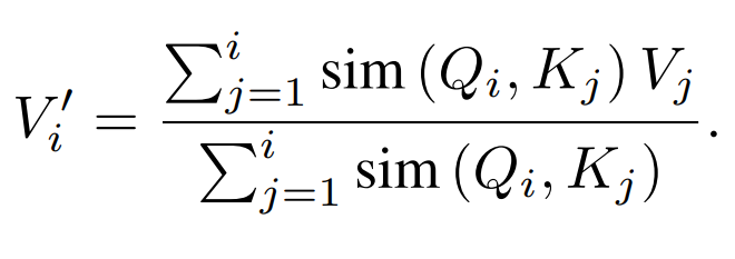
The next work on our list, "Transformers are RNNs: Fast Autoregressive Transformers with Linear Attention" by Angelos Katharopoulos, Apoorv Vyas, Nikolaos Pappas, and François Fleuret, directly builds on the work of our previous paper. They view the efficient attention formulation through the lens of kernel methods and provide an additional implementation of causally-masked autoregressive transformers as RNNs that allows for much more efficient prediction on long-sequences and memory use that is constant with respect to sequence length.

Kernel Interpretation

First, the authors take inspiration from more classical ML (kernel functions) to address the softmax operation in the formulation of QKV attention.  The re-arrangement of the QKV operation that exploits the associativity of matrix multiplication is only valid when there is no softmax applied to the output of \(QK^{T}\) and the operation is linear.  The authors offer a addition of the method from the perspective of kernel methods.

This next section comes with the caveat that as someone self-taught I've remained ignorant of kernel methods for a rather embarrassingly long amount of time – please refer to "Transformer dissection: An unified understanding for transformer’s attention via the lens of kernel" for a vastly more rigorous explanation of this kernel interpretation of attention.

If we have a feature map, \(\phi\), and we're interested in a \((n, n)\) matrix of inner products (in SVM literature, the Gram matrix) of some inputs \(x_i...x_n\) passed through the feature map \(\phi\), there often exists a mathematical shortcut that prevents us from having to ever compute \(\phi(x)\) (which may be very high dimensional and expensive to compute) by directly evaluating some "kernel function", \(k(x_i, x_j)\) for each i, j pair.

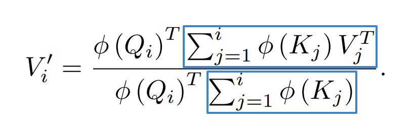
In the case of "Transformers are RNNs", however, this principle is flipped on it's head. They observe that the attention matrix output by \(\text{softmax}(QK^{T})\) looks rather like the Gram matrix of SVM literature, and propose to replace the direct computation of the softmax outputs with \(\phi(Q)\phi(K)^{T}\).  Alongside the re-interpretation with the kernel trick, they apply the same matrix multiplication associativity trick from "Efficient Attention: Attention with Linear Complexities" – producing an attention operation that is indeed linear with respect to sequence length.

Unfortunately the feature space for an exponential kernel is infinite width – which means we can't select a feature map \(\phi\) that exactly reproduces softmax attention.  They experiment with instead using a 2nd-degree polynomial kernel that corresponds to a feature space of size \(d_k^{2}\) for the keys and queries, stating that the polynomial kernel performs similarly to the exponential kernel in practice. This gives us a computational complexity of \(O(n{d_k}^{2}{d_v})\) for the polynomial kernel – which is advantageous when \(d^2 < n\).

They also experiment with a simpler feature map, \(\phi(x) = \text{elu}(x) + 1\), for smaller sequences where the polynomial kernel would typically result in greater computational cost than typical self-attention.  This gives a computational complexity of \(O(n{d_k}{d_v})\).

RNN Interpretation

Up to this point in our discussion of "Transformers are RNNs" we've ignored an important normalizing term for purposes of simplicity, but it represents one final obstacle to efficient inference so we'll re-introduce now. Just like in a softmax operation, regardless of the choise of feature map, it's desirable to normalize by the sum of the attention terms up to index \(i\) such that later terms do not have larger activations.

As we've discussed at length throughout this blog post, the memory complexity of models is often as much of a barrier to operating over long sequences as computational complexity.  In an autoregressive setting, if we have to store the activations of all prior tokens to compute the representation of the next observed token, our memory use will scale necessarily scale linearly with sequence length even though we produce a single token at a time.  This is the case for typical self-attention because we must compute an key-query agreement matrix.

The author's make this possible by:

• Re-organizing the matrix multiplication using the associative property  
• Enforcing causal masking
• Computing running sums of some terms (using custom PyTorch CUDA kernels)

In blue below we denote the running sums – the sum in the denominator we'll refer to as \(S_i\) and the sum in the number we can refer to as \(Z_i\).  At prediction time we just need to add \(\phi(K_j){V_j}^{T}\) to \(S_{i-1}\) and \(\phi(K_j)\) to \(Z_{i-1}\) to compute the next hidden state! The gradient can also be expressed as a cumulative sum, so this memory efficiency trick is also applicable to training time.

After substitution, we have:

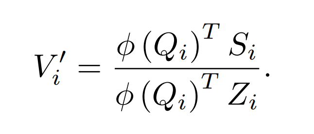
From here, the authors are tantalizingly close to finishing the reformulation as a recurrent model – they need only to define some initial states and write out the recurrence relations and we have ourselves a proper RNN!

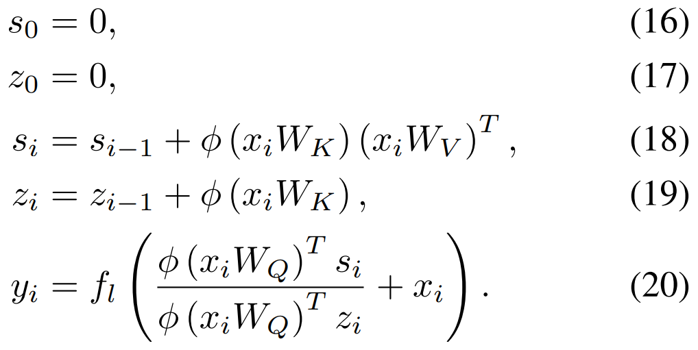
To attempt to layer some of my own intuition over this RNN formulation, I find it helpful to think about:

• \(\phi(x_i W_Q)^{T}\): vector that denotes which of \(d_k\) "channels" are most important for a given input.
• \(s_i\): shape \((d_k, d_v)\), a running summary of information present in each of the \(d_k\) channels.
• \(z_i\): vector of shape \(d_k\) that acts as a normalizing factor, ensuring that the magnitude of each channel's contents does not depend on length.

Experimental Results

Emperical evidence backs up the theory – particularly on runtime and memory benchmarks, the linear attention mechanism proposed by "Transformers are RNNs" shines. The authors focus on image generation and a speech recognition benchmark, but I'd love to see future work that also benchmarks on PG-19 or similar.

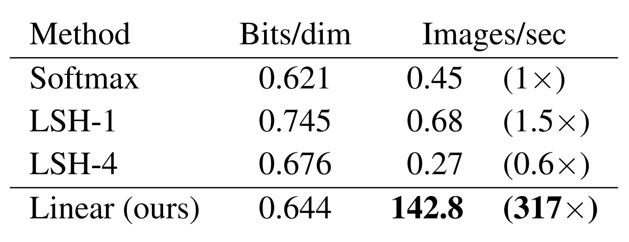
On an MNIST generation task, linear attention posts similar results to softmax attention with >300x faster generation speeds:

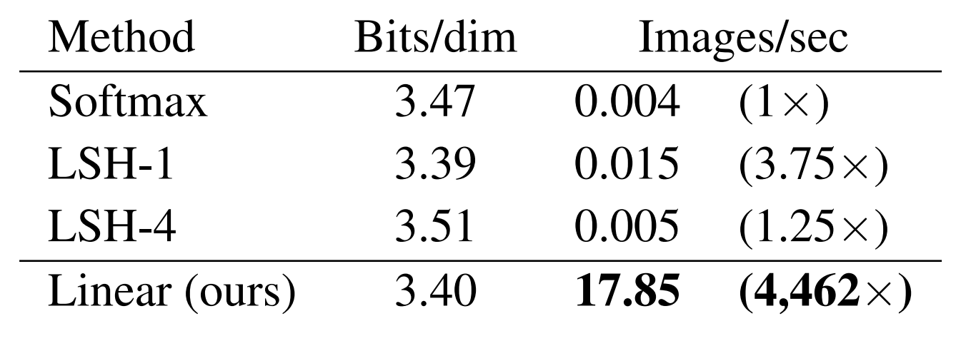
On CIFAR 10 the difference is even more striking:

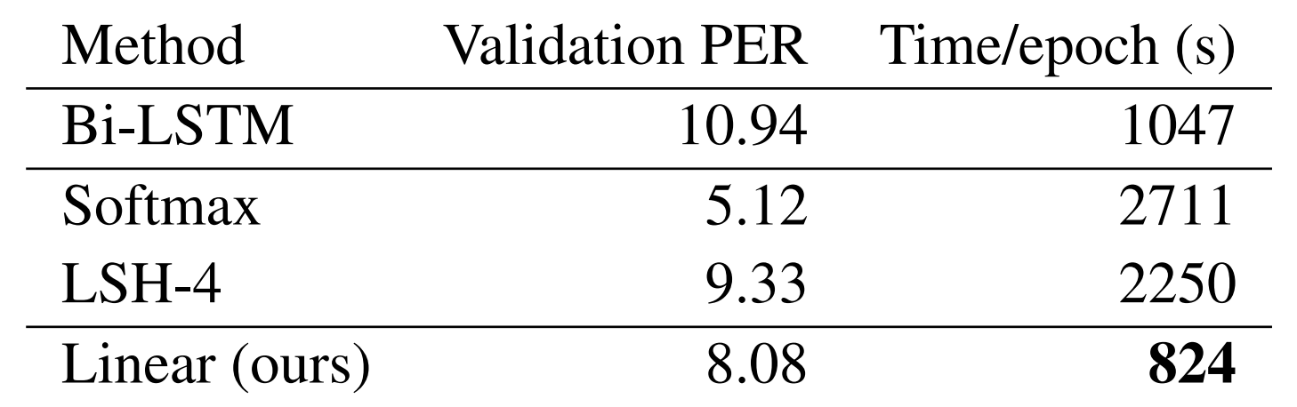
Perplexity on the WSJ automatic speech recognition lags behind softmax attention but still outperforms the Reformer and a Bi-LSTM baseline while also recording faster training times.

To top it all off, this paper sets a high bar for reproducibility in academic research – an explainer video, code with clean high-level wrappers, library documentation, slides, and a colab notebook are all available at https://linear-transformers.com/.

ETC: Encoding Long and Structured Data in Transformers

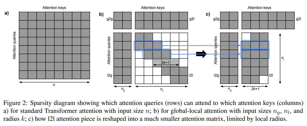
Next up is "ETC: Encoding Long and Structured Data in Transformers", by Joshua Ainslie, Santiago Ontanon, Chris Alberti, Philip Pham, Anirudh Ravula, and Sumit Sanghai.  ETC introduces a concept they call "global-local attention".  In global-local attention, the input is divided into a global part and a local part.  The attention operation itself is then composed of 4 distinct operations – global to global, global to local, local to global, and local to local attention with a fixed size window (also used in works such as the Routing Transformer). In practice these are handled by two separate matrix multiplications – one for global to global + local, and a second for local to global + local (with padding for tokens near the start and end). This attention pattern is visualized in the diagram below.

This structure is a generalization of work previously described in "Star-Transformer" by Qipeng Guo, Xipeng Qiu, Pengfei Liu, Yunfan Shao, Xiangyang Xue, and Zheng Zhang that allows for more than one global token. Like Transformer-XL and other follow up works, they employ relative position embeddings.

The tokens in the global attention don't correspond to actual byte-pair or word-piece tokens – they can be used to represent sentences, paragraphs, or other structured inputs. Then via the use of masking on the global to local attention, the global tokens can be made to explicitly act as summaries of local information and provide higher level representations for subsequent layers to attend to.

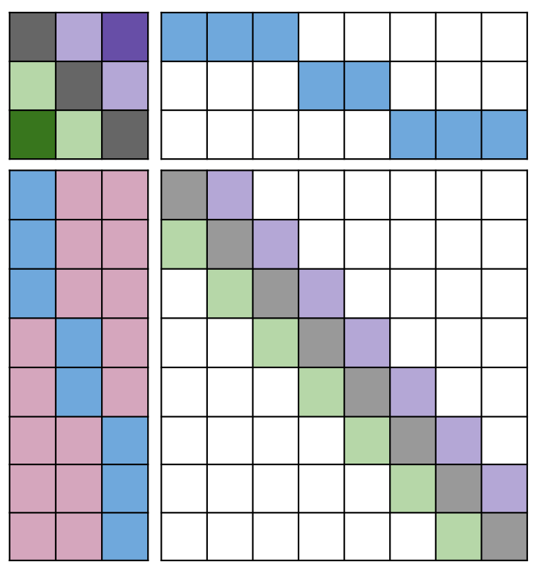
In the diagram below, different colors represent different relative positional embeddings and white represents masking. You'll notice the characteristic local attention pattern in the lower right hand portion of the diagram.  In the upper left (global to global attention), we have a similar relative position pattern but on top of sentence / paragraph summaries. You can see the summary masking in the top right, where global tokens only attend to a structured subset of the input sequence that corresponds to a unit of the input like a sentence or paragraph. Finally, in the lower left the local tokens in this setup attend strongly to a subset of the global tokens that aligns with their subset of the input sequence (in blue) and less strongly to summary information from other global tokens.

Importantly nothing requires use to use the global attention to represent sentences or paragraphs.  We could use the global attention without any structured attention pattern over the input sequence, or represent items that have no apparent order by keeping the relative position embeddings in the local to global attention constant. ETC presents a general framework for incorporating our own inductive biases via decisions about relative position embeddings and input masking.

Computational Complexity

Computational complexity for the ETC model depends on the size of the global attention and the size of the local window, \(k\). For global size \(n_g\) and local size \(n_l\), memory and computational complexity are both \(O(n_g^{2} + n_g n_l + k n_l)\). In practice the computational cost is dependent on the granularity of the global units (sentences, paragraphs, pages, etc).  

Experimental Results

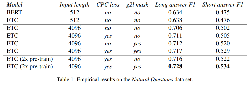
The authors benchmark their method on the Natural Questions dataset. Even without additional modifications like the addition of a CPC loss as part of the model's pretraining process, they observe a ~8 F1 point gap between BERT and and ETC model trained on an input sequence of length 4096 with global size of 230 and local window size of 84 tokens on either side.

Similar Work

In a similar vein to ETC, Ankit Gupta and Jonathan Berant of Tel Aviv University extend transformers with a global memory mechanism in their work "GMAT: Global Memory Augmentation for Transformers".  Distinct from the scenarios explored ETC, the global memory tokens in GMAT do not correspond to sentences or paragraphs and attend to every element of the input sequence rather than providing any explicit structure in the attention patterns of the global memory. They show promising initial results on tasks from masked language modeling to sequence compression to reading comprehension.

Longformer

AllenAI's Iz Beltagy, Matthew E. Peters, and Arman Cohan also propose the use of a global memory mechanism independent of sequence length in their work "Longformer: The Long-Document Transformer". Unlike ETC and GMAT where global attention tokens do not correspond to literal lexical units from the source document, the Longformer's long-term memory mechanism denotes a fraction of all actual input tokens to be part of the global memory in a per task manner.

For classification tasks, for instance, only the [CLS] token is part of the global memory, and the Longformer ends up looking rather similar to the star-transformer, where long-term interactions are likewise all routed through a single token. For question answering, all question tokens are part of the global memory.  

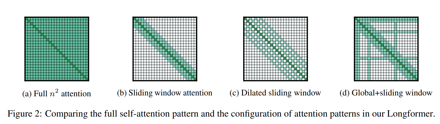
Projections for the global memory representations are learned independently from typical key, query, and value projections.  In addition to a global memory mechanism, the Longformer architecture employs local sliding window attention like many of the other papers on our list.  Similar to OpenAI's Sparse Attention, they also use a dilated attention pattern to help capture longer term interactions at lower computational cost.

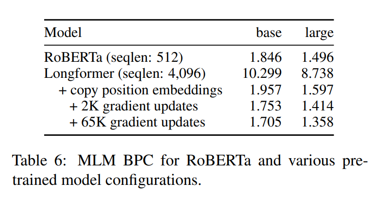
Perhaps the most novel contribution of the Longformer is the initialization scheme – they cleverly copy the weights of RoBERTa and duplicate the absolute position embeddings 8x of RoBERTa large in order to support sequences of up to 4096 tokens in length (rather than the typical 512), then continue pretraining with the masked language modeling objective for 65k gradient updates.  

Thanks to their initialization from the RoBERTa checkpoint, the model already achieves ~1.96 BPC (compared to RoBERTa's 1.85) on a combination of the Books Corpus, English Wikipedia, Realnews, and Story Corpus at initialization. It quickly learns to make use of the new attention patterns and larger context size and surpasses the 1.85 baseline in <2K gradient updates.

Experimental Results

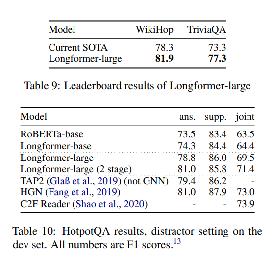
Contrary to many of the other papers we've explored, the Longformer mainly aims to show the utility of attending to a longer context rather than focusing on the efficient use of longer contexts, so many of the hyperparameter settings used in their experiments are substantially more expensive that the RoBERTa baseline.

However, this work does an excellent job of motivating the use of longer context lengths, and achieves current SOTA on both Wikihop and TriviaQA while also posting competitive scores on HotPotQA although many other top-performing models include more task-specific architectural modifications.

An implementation of the Longformer is available as part of the HuggingFace transformers package or independently through the AllenAI github.

Other Approaches To Long Term Context in Transformers

If you're interested in other approaches to incorporating long-term context in transformers, you might also enjoy reading:

• A Cheap Linear Attention Mechanism with Fast Lookups and Fixed-Size Representations
• Adaptively Sparse Transformers
• Blockwise Self-Attention for Long Document Understanding
• BP-Transformer: Modelling Long-Range Context via Binary Partitioning
• Residual Shuffle-Exchange Networks for Fast Processing of Long Sequences
• Synthesizer: Rethinking Self-Attention in Transformer Models
• Deep Equilibrium Models
• Scaling Laws for Neural Language Models
• Multi-scale Transformer Language Models
• Big Bird: Transformers for Longer Sequences

Did I miss a paper you think should have been included or misinterpret a key detail? Send me your suggestions and corrections on twitter or reach out directly to madison@pragmatic.ml.